A thermal imaging camera has been used to view a target at night for military purposes for the past 40 years. In recent times, civilian demands for the thermal camera have been gradually increasing. Civilian demands are primarily in the security, industry, research and medical fields. The thermal imaging camera measures the radiation of the target, and the measured radiation can be expressed by the distribution of the radiative temperature [1]. It is often necessary for optical systems to have multiple fields of view. A zoom system can have continuous changes of the field of view by moving lens groups along an optical axis.
In this paper, paraxial studies and lens modules are used to obtain the optimum initial design of a 10× extended four-group inner-focus zoom system for an LWIR camera. It is integrated into uncooled IR detectors with 384×288 pixels, of which pixel size is 25 µm. The f-number of the optical zoom system was estimated to be F/1.4 from the Airy disk and MRTD(Minimum Resolvable Temperature Difference) analysis [2-5].
Through an optimization process, we have obtained an optical zoom system satisfying the requirements for a 10× LWIR camera. In order to balance the wave front aberrations, we located the diffractive surfaces at L3 and L6. Since the diffractive lenses are designed to be very weakly powered and the wavelength to zone period ratio is very small across the entire lens, the scalar predictions of diffraction efficiency are valid to calculate the polychromatic integrated diffraction efficiency. The changes of the MTF(Modulation Transfer Function) due to diffraction efficiency are evaluated from the polychromatic integrated efficiency [6].
II. OPTICAL DESIGN REQUIREMENTS
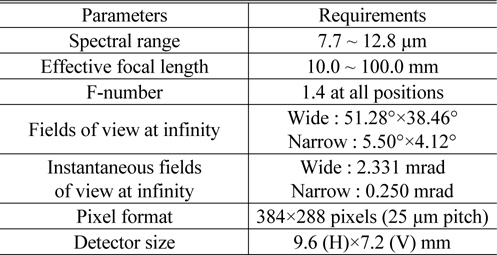
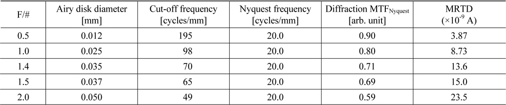
The main requirements of an LWIR zoom system are listed in Table 1. Since the f-number has an effect on Airy disk diameter as well as on MRTD, the optical system with uncooled IR detector should have a low f-number, if possible [7]. Basically spatial resolution of an IR optical system is decided by the specification of IR detector, because target acquisition performance is based on the number of line pairs resolvable across a target critical dimension. Consequently an IR optical system should be designed to have the diffraction limited performance [3].
[TABLE 1.] Optical requirements for a LWIR zoom system

Optical requirements for a LWIR zoom system
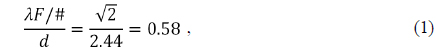
The Airy disk diameter is given by 2.44·λ·F-number. In diffraction limited system, a pixel’s diagonal size of detector should be equal to the Airy disk diameter as follows:
where
The MRTD is one of the criteria denoting optical system performances, which characterizes the thermal sensitivity at a given spatial frequency [8], whereas the MTF measures the attenuation in modulation depth without regard for thermal property of an object. This MRTD is given by

where
[TABLE 2.] F-number versus MRTD
F-number versus MRTD
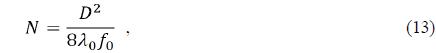
Since the diffraction MTF depends on the f-number of an optical system, a large f-number results in a large value of MRTD, which reduces the resolution for resolvable temperature difference. Meanwhile, a small f-number gives a good value of MRTD, however, the large aperture system is limited by the cost and the detector. From the exact evaluation for the relationship between f-number and MRTD, optimum f-number of this system is confirmed to be 1.4. The MRTD at F/1.4 is so small that it may give enough resolution.
III. INITIAL DESIGN FOR AN LWIR ZOOM SYSTEM
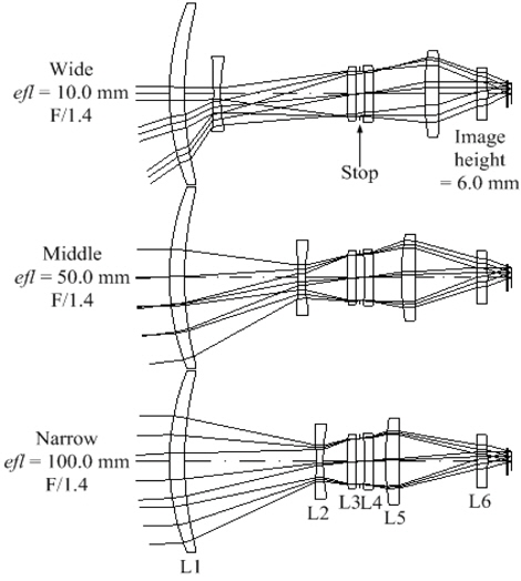
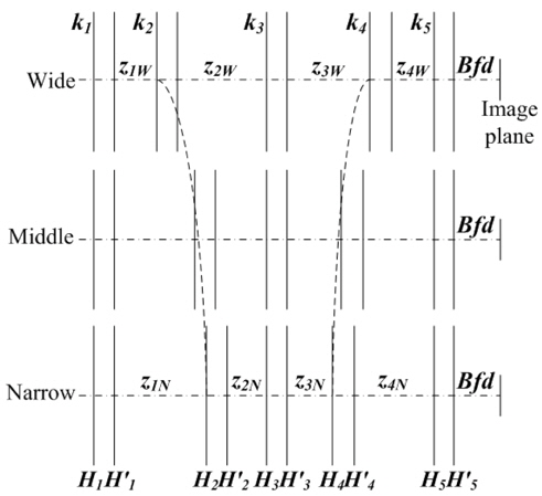
Figure 1 illustrates an extended four-group inner-focus zoom system that has the same total track length at all zoom positions. The zoom system is composed of fixed three groups, the second group for zooming, and the fourth group for focusing.
The powers of the groups are denoted by
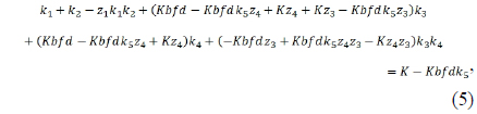
We can analytically derive the set of zoom equations for an extended four-group inner-focus zoom system with infinite object by using the Gaussian brackets. The initial design of this zoom system can be formulated as follows [10-12]:


where

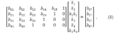
Therefore, Eqs. (5) and (6) can be expressed in a matrix form at wide and narrow field positions as follows:

where
where


Inserting the conditions of Eqs. (9) ~ (11) into the first row equation of Eq. (8) results in an expression for the unknown parameter

where
For the initial design of a 10× extended four-group inner-focus system, we input the proper distances between principal points and the targeted total powers at wide and narrow positions. These starting values of z1, z2, z3, z4, and
[TABLE 3.] The starting parameters for zoom loci (in mm)
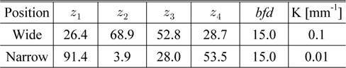
The starting parameters for zoom loci (in mm)
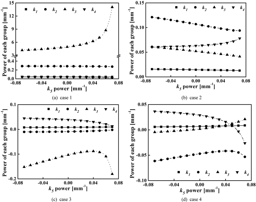
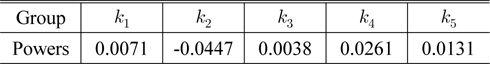
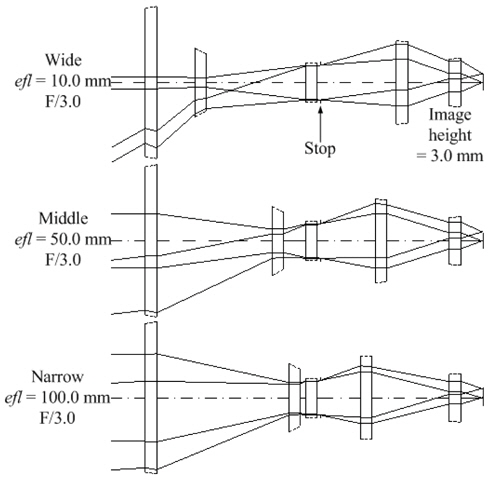
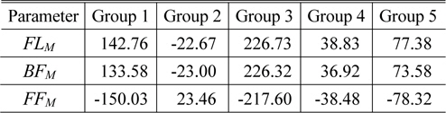
By inputting these starting values of Table 3 into Eqs. (5) and (6), we can obtain the proper values for the power of each group from Eqs. (9) ~ (12). Figures 2 illustrates the four solution sets of Eq. (12) for various
In the solutions of case 1 and case 2, the powers of the second group (
Finally, the solutions of case 4 satisfy the requirements for power distribution available to our zoom system having zoom ratio of 10×. Among the solutions of case 4, we took the powers of
[TABLE 4.] Paraxial design data for the powers (in mm-1)

Paraxial design data for the powers (in mm-1)
We have set up a zoom lens system with five thin-lens modules, for which the power of each group and the zoom locus inputs are taken from Table 4 and Table 3. The lens modules do not reflect higher-order aberrations, so reducing the aperture and the field size of the system is desirable [13, 14]. Thus, we took a zoom system with a half image size of 3 mm and f-number of F/3 at all positions. The air distances between modules were constrained to be longer than 3.0 mm for the mounting space.
In Table 3 and Table 4 of the previous paraxial study, the thickness of each group and the air spaces are not presented. They can be derived by specifying the design variables of the lens modules, such as the effective focal length (
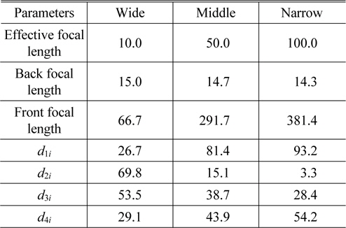
First-order properties and zooming loci of the zoom system consisting of five thick lens modules (in mm)
[TABLE 6.] Design data for the lens modules in the optimized lens module zoom system (in mm)

Design data for the lens modules in the optimized lens module zoom system (in mm)
A real lens group is generally composed of several lens elements, which should be equivalent to the lens module given in Table 6. In this paper, an optimization design method is used to design a real lens group equivalent to the module of each group. We choose an appropriate structure for each real lens group and scale it up or down so that the focal length of each real lens group is the same as that of the lens module. By using the optimization method of Code-V, we matched the first-order quantities of the lens module to those of a real lens. For the conversion process, the design variables of the real lens are the radius of each surface, the thickness, and the refractive index. Therefore, the three constraints given in Table 6 can be satisfied by specifying the lens design variables. After a few iterations, the real lenses of the groups are obtained.
If a zoom system equivalent to the lens module zoom system is to be achieved, the air spaces (
IV. OPTIMIZED DESIGN FOR A ZOOM SYSTEM USING DIFFRACTIVE LENSES
In the initial design of the zoom system, we reduced the aperture and the field size so that they were too small. If current specifications for an LWIR zoom camera are to be met, the aperture and the field size should be increased. The f-numbers are extended to
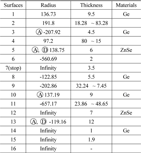
[TABLE 7.] Design data of an optimized zoom system (in mm)

Design data of an optimized zoom system (in mm)
This system consists of the six lenses including two diffractive surfaces. The diffractive surfaces are used to balance the wave-front aberrations. They are located in the front surface of L3 and the back surface of L6. The hybrid lenses such as L3 and L6 have refractive and diffractive properties at the same time. Therefore the hybrid lens differs from a conventional refractive lens in that it can produce many images due to diffraction orders. These diffraction images serve to lower the contrast of the desired image.
The rotationally symmetric diffractive lens has the surfacerelief of ring type. The number of rings (

where
[TABLE 8.] Specifications of the hybrid lenses (in mm)
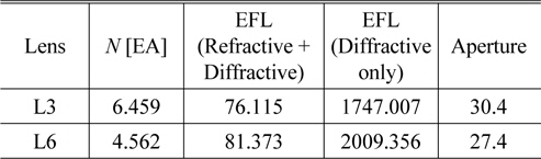
Specifications of the hybrid lenses (in mm)
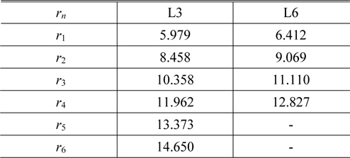
[TABLE 9.] The radius of each zone rn (in mm)

The radius of each zone rn (in mm)
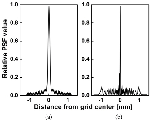
Figure 5 compares two point spread functions by L3, Fig. 5(a) is obtained from refracted image only and Fig. 5(b) from refracted plus diffracted images. Other diffraction orders, not design order, generate the background noises such as flares. They result in degrading the contrast at around zero frequency. However, the width of the central peak is much more narrow than that of the refracted image, which eventually improves the image quality at high frequency.
For a diffractive optical system that utilizes spectrally broadband illumination, the wavelength dependence of diffraction efficiency needs to be considered when evaluating imaging performance. To determine the polychromatic transfer function for a diffractive lens, it is first to define a polychromatic integrated efficiency for the wavelength band ranging from λmin to λmax. Denoting the integrated efficiency at wavelength λ by
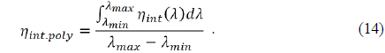
In Table 8, the diffractive components are very weakly powered, to the 4 % of the hybrid component’s powers. In addition to that, the wavelength to zone period ratio is very small across the entire lens, as shown in Table 9. In these situations, it is known that scalar predictions of diffraction efficiency are valid to replace the

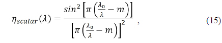
where λ0 is the design wavelength for the diffractive lens. The expression for
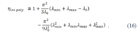
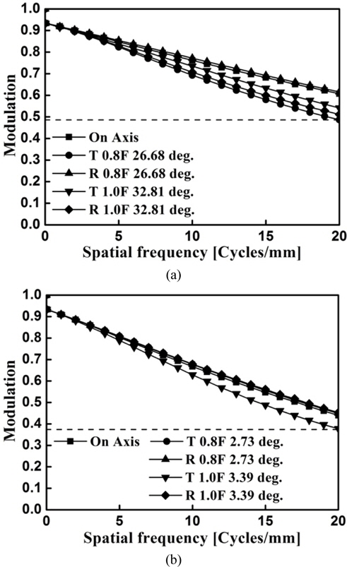
As a result, the polychromatic integrated efficiency of an LWIR zoom system is 93.39 % and background noise reduces the diffraction efficiency by 6.61 % for λmin = 7.7 µm, λmax = 12.8 µm, and λ = 10.2 µm. These losses in diffraction efficiency may reduce the contrast of image. Figure 6 shows the polychromatic modulation transfer functions calculated by using the Eq. (16). The polychromatic MTF is scaled by and drops down at zero-frequency. The resulting curves show the behavior predicted by point spread functions of Fig. 5(b).
We have designed and evaluated the optical zoom system for an LWIR camera with an uncooled IR detector. The fields of view are 51.28° × 38.46° at wide and 5.50° × 4.12° at narrow field positions. The optimum f-number of the zoom system was determined to be F/1.4 from Airy disk and MRTD analysis.
Through paraxial design and optimization method, we have obtained an extended four-group inner-focus zoom system having a focal length of 10 to 100 mm. Balancing the wave-front aberrations by use of diffractive surfaces, we improved the performance of the zoom system further. To evaluate the polychromatic transfer function for a weakly powered diffractive lens, the scalar diffraction theory was effectively used.
As a result, the polychromatic integrated efficiency is 93.39% and background noise reduces the diffraction efficiency by 6.61%. This loss in diffraction efficiency slightly reduced the contrast of image at zero-frequency, and scaled down the polychromatic MTF by . However, the designed optical zoom system has enough image qualities for an LWIR camera, as shown in Fig. 6. Consequently, the zoom system developed in this work performs reasonably as an LWIR zoom camera.