Regression and pattern classification are very widely used in many fields and applications.1 Both face four major challenges: 1) choosing the variables/features; 2) choosing the nonlinear structure of the regressors/discriminant functions; 3) choosing how many terms to include in the regression model/pattern classifier; and, 4) optimizing the parameters that complete the description of the regression model/pattern classifier.

For Challenge 1, how to choose the variables/features is crucial to the success of any regression model/pattern classifier. In this paper we assume that the user has established the variables that affect the outcome, using methods already available for doing this. For Challenge 4, there are a multitude of methods for optimizing parameters, ranging from classical steepest descent (back-propagation) to a plethora of evolutionary computing methods (e.g., simulated annealing, GA, PS0, QPSO, ant colony, etc. [4]), and we assume that the user has decided on which one of these to use. Our focus in this paper is on Challenges 2 and 3.

For Challenge 2, in real-world applications the nonlinear structures of the regressors/ discriminant functions are usually not known ahead of time, and are therefore chosen either2 as products of the variables (e.g., two at a time, three at a time, etc.), or in other more complicated ways (e.g., trigonometric-, exponential-, logarithmic-functions, etc.). Sometimes knowledge about the application provides justifications for the choices made for the nonlinear terms; however, often one does not have such knowledge, and a lot of time is spent, using trial and error, trying to establish the nonlinear dependencies. For Challenge 3, how to determine how many terms to include in the regression model/pattern classifier is also usually done by trial and error, and this can be very tedious to do. In this paper we present a novel method that chooses the nonlinear structure of the regressors/discriminant functions as well as the number of terms to include in the regression model/pattern classifier simultaneously and automatically. This is accomplished using a novel way of pre-processing the given data.

The rest of this paper is organized as follows: Section 2 explains how data can be treated as cases; Section 3 explains how each variable must be granulated; Section 4 describes the Takagi-Sugeno-Kang (TSK) rules that are used for regression/ pattern classification; Section 5 presents the main results of this paper, a novel way to simultaneously determine the nonlinear structure of the regressors/discriminant functions and the number of terms to include in the regression model/pattern classifier; Section 6 provides some discussions; and, Section7 draws conclusions and indicates some directions for further research.

A data pair is denoted (x(t), y(t)) where x=col(x₁, x₂, ..., x_p), x_i is the i^th variable/feature and y(t) is the output for that x(t). As is commonly done in the social sciences [5, 6], each data pair is treated as a “case” and index t denotes a data case. Treating data as cases is motivated by a method called fuzzy set qualitative comparative analysis (fsQCA), which was developed by the prominent social scientist Ragin [5, 6], and has been thoroughly quantified by Mendel and Korjani [7, 8].

Note that there may or may not be a natural ordering of the cases over t. In multi-variable function approximation or pattern classification applications the data have no natural ordering; but in time-series forecasting applications the data cases have a natural temporal ordering. We assume that N data pairs are available, and refer to the collection of these data pairs as S_Cases, where

To begin, each of the p variables is granulated [9] into a fixed number of terms. Our suggested approach is to begin with only two terms per variable, design the regression model/pattern classifier, and determine if acceptable performance is obtained. If it has not, then increase the number of terms to three (then four, etc.) and repeat this process, stopping when acceptable performance has been obtained. Due to space limitations, we explain our preprocessing only for two terms per variable. Its extensions to more than two terms is straightforward.

For illustrative purposes, we shall call the two terms high (H) and low (L). Each variable x_i (i = 1, …, p), x_i ∈ R⁺ (or x_i ∈ R), is mapped into the membership functions (MFs) of two type-1 fuzzy sets, one each for high and low. There are many different ways to do this, e.g. choose each MF as a prescribed two-parameter sigmoidal or piecewise-linear function.

In order to use the construction that is described in Section 5, it is required that the two MFs must be the complement of one another. This is easily achieved by using fuzzy c-means (FCM) for two clusters [10], (or linguistically modified FCM [LM-FCM] [11]), because it is well known that the MFs for the two FCM clusters are constrained so that one is the complement of the other.

As a result of this preprocessing step, the MFs 𝜇_Li(x_i) and 𝜇_Hi(x_i) = 1 −𝜇_Li(x_i)(i = 1, ..., 𝑝) will have been obtained. Note that, if independent MFs are used for L_i and H_i(for which 𝜇_Hi(x_i) ≠ 1–𝜇_Li(x_i), then our Section 5 method will use L_i and H_i as well as their complements−four quantities. When, however, 𝜇_Hi(x_i) = 1 −𝜇_Li(x_i) the four quantities reduce to two.

Our rules for a rule-based regression model or classifier have the following TSK structure [12]:

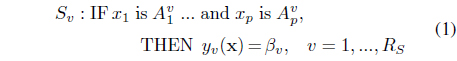
For the rule-based regression model, the β_𝜐 play the role of the regression coefficients which are determined by means of optimizing a regression objective function (e.g., minimizing a root mean square error), whereas for a binary pattern classifier the β_𝜐 are either +1 or -1, depending upon which class the rule is for. Regardless of whether Eq. (1) is used for regression or pattern classification, observe that the antecedent structure (x₁ is … and x_p is ) and the number of rules (R_S) must be specified, after which it is straightforward to convert Eq. (1) into a so-called fuzzy basis function expansion [12, 13]. It is the mathematics of this conversion that establishes the nonlinear natures of the regressors/discriminant functions (Challenge 2); but this requires determining R_S and the antecedent structure. We show how to determine these simultaneously and automatically in the next section.

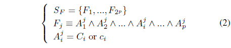
The (compound) antecedent of each rule contains one linguistic term or its complement for each of the p variables, and each of these linguistic terms is combined with the others by using the word “and” (e.g., A₁ and A₂ and … and A_p). We refer to this interconnection as a causal combination3. Note that in a traditional if-then rule the antecedents only use the terms and not their complements. In our approach (as in fsQCA), protection about being wrong for postulating a term is achieved by considering each term as well as its complement.

To begin, 2^𝑝 candidate causal combinations (the 2 is due to both the term and its complement4) are conceptually postulated (we will show below that these causal combinations do not actually have to be enumerated). If, e.g., 𝑝 = 6 there would be 64 candidate causal combinations, or, if 𝑝 = 10, there would be 1,024 candidate causal combinations.

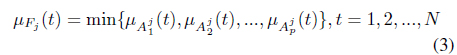
One does not know ahead of time which of the 2^𝑝 candidate causal combinations should actually be used as a compound antecedent in a rule. Our approach prunes this large collection by using the MFs that were determined in Section 3, as well as the MF for “A₁ and A₂ and… and A_𝑝” (obtained using fuzzy set mathematics) and a simple test. The results of doing this are called R_s surviving causal combinations.

Let S_F be the collection of the following 2^𝑝 candidate causal combinations, F_j (j = 1,…, 2^𝑝 and i = 1, …, 𝑝):

where ∧ denotes conjunction (the “and” operator) and is modeled using minimum and (using Ragin’s [5] notation) c_i denotes the complement of C_i. The R_S surviving causal combinations are found from all of the 2^𝑝 candidate causal combinations by keeping only those causal combinations whose MF > 0.5 for at least f cases, where f is a threshold that has to be specified ahead of time5. A brute force way to do this is to create a table in which there are N rows, one for each case, and 2^𝑝 columns, one for each of the causal combinations. The entries into this table are μ_Fj (t) and there will be N2^𝑝 such entries. Such a table is called a truth table by Ragin [4, 5]. One then searches through this very large table and keeps only those causal combinations whose MF entries are > 0.5. If f = 1 then all such causal combinations, removing duplications, become the set of R_S surviving causal combinations. It is very easy for N2^𝑝 to become very large6 and so this brute force way to carry out this procedure is impractical.

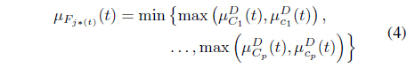
Ragin [5] observed the following in an example with four causal conditions: “... each case can have (at most) only a single membership score greater than 0.5 in the logical possible combinations from a given set of causal conditions (i.e., in the candidate causal combinations).” This somewhat surprising result is true in general and in [8] the following theorem that locates the one causal combination for each case whose MF > 0.5 was presented:

Theorem 5.1 (min-max theorem). [8]: given p causal conditions, C₁, C₂,…, C_𝑝 and their respective complements, c₁, c₂, …, c_𝑝. Consider the 2^𝑝 candidate causal combinations (j = 1, …, 2^𝑝) where or ci and i = 1, …, 𝑝.

Proof. Let

Then for eacht (case) there is only one j, j * (t), for which 𝜇_Fj*(t) (t) > 0.5 and 𝜇_Fj*(t) (t) can be computed as:

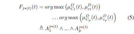
where is determined from the right-hand side of Eq. (4), as:

In Eq. (5), arg max denotes the winner of max namely C_i or c_i.

A proof of this theorem is in [8]. When n_c independent terms are used for each variable, replace p by n_cp. A numerical example that illustrates the computations can be found in [7].

This min-max Theorem leads to the following procedure for computing the R_S surviving causal combinations7:

1. Compute F_j＊(t) using Eq. (5).

2. Find the J uniquely different F_j＊(t) and re-label them F_j′ (j^′ = 1, …, J).

3. Compute t_Fj′, where (t = 1, …,N)

4. Compute N_Fj′, where

5. Establish the R_S surviving causal combinations (𝜐 =1. …,R_S), as:

where F_j′ (j^′ → v) means F_j′ is added to the set of surviving causal combinations as , and v is the index of the surviving set.

Numerical examples that illustrates this five-step procedure can be found in [8].

In order to implement Eq. (8) threshold fhas to be chosen. In our works, we often choose f = 1. This choice is arbitrary and depends on an application and how many cases are available. Discussions on how to choose f are given in [5-7, 14]. One popular way to choose f is as the integer such that at least 80% of all cases are covered by the set of surviving causal combinations.

From F_j in Eq. (2) and in Eq. (8), it follows that (v = 1, …, R_S):

In [8] it is shown that the speedup between our method for determining the surviving causal combinations and the bruteforce approach is ≈ O (2^n_cp), where n_c is the number of terms used for each variable (assumed to be the same for all variables).

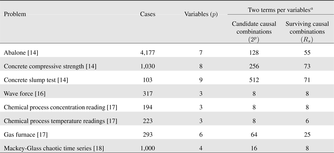
Example: This example illustrates the number of surviving causal combinations for eight readily available data sets: abalone [15], concrete compressive strength [15], concrete slump test [15], wave force [16], chemical process concentration readings [17], chemical process temperature readings [17], gas furnace [17] and Mackey-Glass Chaotic Time Series [18]. Our results are summarized in8 Table 1. For each problem a two-cluster FCM was applied to all of its cases. The five-step procedure described above was then used to determine R_S.

Observe that: (1) for three variables (as occurs for wave force, chemical process concentration reading and chemical process temperature readings), the number of surviving causal combinations is either the same number, or close to the same number, as the number of candidate causal combinations, which suggests that one should use more than two terms per variable; and, (2) In all other situations the number of surviving causal combinations is considerably smaller than the number of candidate causal combinations. Although not shown here, this difference increases when more terms per variable are used, e.g., using three terms per variables the candidate causal combinations for the concrete slump test data set is 134,217,728 whereas the number of surviving causal combinations is only 97 [19].

Observe, from the last column in Table 1, that for four of the problems R_S ≥ 25. We seriously doubt that a human designer could postulate the non-linear structures for so many regressors/discriminant functions. Our method not only shows that so many of them are necessary, it also finds their nonlinear structures.

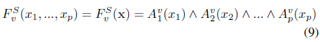
In Korjani and Mendel [19] have shown how the surviving causal combinations can be used in a new regression model, called variable structure regression (VSR). Using the surviving causal combinations one can simultaneously determine the number of terms in the (nonlinear) regression model as well as the exact mathematical structure for each of the terms (basis functions). VSR has been tested on the eight small to moderate size data sets that are stated in Table 1 (four are for multi-variable function approximation and four are for forecasting), using only two terms per variable whose MFs are the complements of one another, has been compared against five other methods, and has ranked #1 against all of them for all of the eight data sets.

Specific formulas for fuzzy basis function expansions can be found in [12, 13]. Similar formulas for rule-based binary classification can be found in [12].

Surviving causal combinations have also been used to obtain linguistic summarizations using fsQCA [7, 8].

This paper presents a novel method for simultaneously and automatically choosing the nonlinear structures of regressors or discriminant functions, as well as the number of terms to include in a rule-based regression model or pattern classifier. Variables are first partitioned into subsets each of which has a linguistic term (called a causal condition) associated with it; fuzzy sets are used to model the terms. Candidate interconnections (causal combinations) of either a term or its complement are formed, where the connecting word is AND which is modeled using the minimum operation. The data establishes which of the candidate causal combinations survive. A novel theoretical result leads to an exponential speedup in establishing this. For specific applications, see [7, 8, 19].

Much work remains to be done in using surviving causal combinations in real-world applications. The extension of the min-max Theorem to interval type-2 fuzzy sets is currently being researched.

No potential conflict of interest relevant to this article was reported.