At least since the economical crisis the traditional way of designing ships is considered to be outdated. Operating ships at off-design conditions may appear as a good solution in times of a crisis and apparently leads to lower fuel consumption but there is a potential to save even more energy if the vessels would have been designed with respect to more operational conditions. But even without the crisis the process of designing a ship onto one operating condition had to be reconsidered, for the fact that both calculations or prognosis as done by Røe (2010) and analyses of operating profiles of real ships have shown that merchant vessels only operate at their respective design condition (e.g. at 85% Maximum Continuous Rating (MCR)) for a small amount of time.
Despite this fact, the knowledge of a vessels future operational profile is of great interest when it comes to environmental issues as a suboptimal ship design has a higher emission rate than an optimal one.
These problems necessitate a new approach which is capable to deal with future needs and uncertainties and which considers the vessels life-long operating situation. Keeping that in mind, scenario methods seem to be a suitable solution. By linking economical trend analysis with detailed operation profiles the usage of these methods offers the possibility to design ships which are not optimized to one or two particular operational conditions but will be significantly more efficient related to their overall operating time.
The idea of using a complete operational profile as the basis for the development or optimization of a hull form instead of a single or only a few design points has been adapted within a few projects before. Two of them are in short presented in the following.
As an example, Temple and Collette (2012) have been using probability density functions in order to display the speed range of two vessels (DTMB-5145 naval combatant and KCS container ship) for a following multi-objective optimization of their hull forms. The optimization is done using a Multi-Objective Genetic Algorithm (MOGA) with the lifetime resistance being calculated from the integral over the speed dependant total resistance (estimated using the thin ship theory) multiplied by the Probability Density Function (PDF). The respective PDFs have been generated by applying a bimodal distribution with the two modes representing the vessel’s endurance and mission speed in case of the DTMB-5145 and an unimodal distribution with the mode at the vessels design speed for the KCS. As far as the author is aware, those distribution functions are not based on statistics of existing vessels but on the author’s consideration.
Statistically based probability distribution functions have been used by Eljardt (2010) in order to assess different vessel types, shipping routes or the commodity flow. Despite the speed distribution, he also considers environmental data such as seastate and wind conditions and other vessel specific data, e.g. the trim. Thereby, the respective distribution functions are taken from statistical analysis and / or prognosis. Within this work the distribution functions are used for sampling a sufficient number of ship operation conditions using the Monte Carlo Method in order to serve for example as the target function for an optimization of a ship’s hull form and propulsion system. Although considering a wide range of parameters, this approach differs to the scenario based approach presented in this paper as it does not completely consider the coupled or correlated appearance of different parameters, which can lead to incorrect results in the target function (see next section for details).
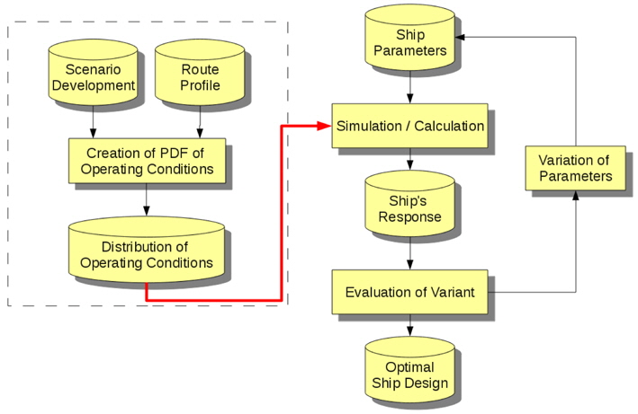
The basic idea of the scenario based approach is to predict the most probable operating conditions the designated vessel will stay in during its operating time in order to find the most suitable design variant. Fig. 1 shows the flow chart of the complete optimization process as presented in Wagner and Bronsart (2011).
It can be seen, that the general procedure can be divided into two stages. The first stage consists of the development of a probability density function of operating conditions on the basis of a given route profile and specific scenario development functions. Based on this distribution a target function can be derived, which consecutively will be handed over to stage two - a traditional hull form optimization process chain - in order to evaluate an optimal design variant. As the methodology of the second stage can be considered to be well known, this paper mainly focuses on the part of the scenario creation.
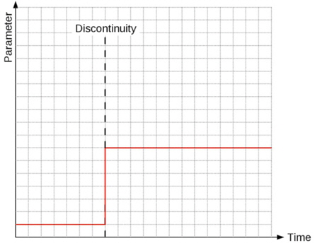
In order to meet the claim of developing a distribution of operating conditions and subsequently from this deriving the target function, a basic operational profile consisting of a chronological sequence of ship operating parameters will be projected into the future by reiterating it several times. This leads - as a simplified example only considering one unspecific parameter - to the picture given in Fig. 2.
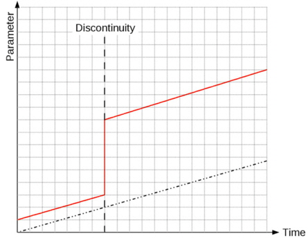
To represent constantly changing surrounding parameters one or more development functions are added to the reiterated data. Continuing the above example and with a constant linear development function indicated by the dotted line the picture given in Fig. 3 develops.
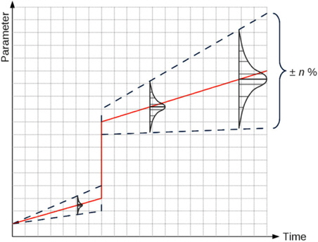
As the forecasted development functions normally are afflicted with insecurity, gradually increasing uncertainties in form of a normal distribution of probabilities will be added to the sequence. In Fig. 4 it can be seen, that at this point the probability of any possible value of a parameter P can be determined at any certain point in time T, allowing to sum up the respective probabilities of all operating situations the vessel will possibly stay in during its life-time.
From the resulting Frequency Distribution (FD) of operating conditions the most probable ones can be chosen in order to serve as a basis for an optimization considering more than just one operating condition.
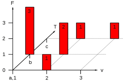
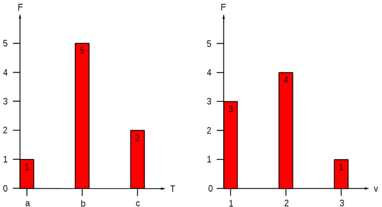
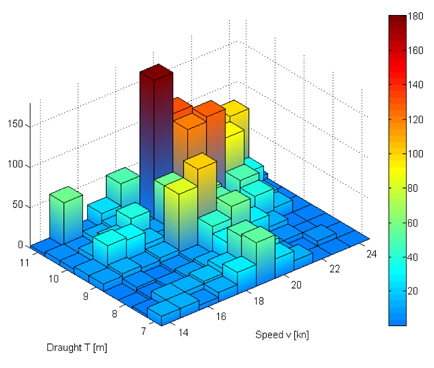
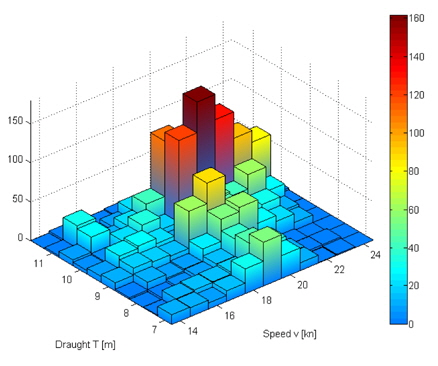
In case of more than one observed parameter one advantage of this approach against for example the Monte Carlo sampling of distribution functions of single parameters as done in Eljardt (2010) exists in the consideration of coupled appearances of different parameters. Fig. 5 shows the coupled exemplary distribution of speed (1 to 3) and draught (a to c) values of a vessel with the main peak at speed 1 and draught b, followed by speed 2 and draught b. Deriving the single parameter distribution results in the diagrams given in Fig. 6. It can be seen, that - when sampling these two diagrams - the designer would most probably come to the wrong conclusion, that the main operating condition is the combination of speed 2 and draught b. Although this problem can be solved for the Monte Carlo Method by the identification of correlations and the implementation of conditional probabilities, this approach can become time consuming, especially with a further increasing number of parameters. With an increasing complexity of the system, the direct modeling of the scenario approach becomes comparatively easier and will in most cases also be more accurate.
In the following the functionality of this optimization approach is presented using the example of the bulbous bow of the KCS.
To have a realistic basis to start with, the log-data of an existing comparable 3600
As it covers approximately a time span of three years and eight months including the beginning of the economical crisis this data have been considered to represent a typical picture of today’s vessels operating situation. When choosing bin sizes of 1 knot for the vessels speed and 0.5
As it is intended to not only consider the past but also the future, the existing data have been put into a loop covering a time span of approximately eleven years. In order to consider a possibly changing transport task due to changing economical conditions, assumptions regarding the possible future development of the global economy have to be done. For convenience reasons constant linear growths for all loops have been chosen as follows:
• Loop 1: -0.5% per year (decrease). • Loop 2: 0% per year (stagnation). • Loop 3: 0.5% per year (increase).
Subsequent a translation of these surrounding conditions to the floating condition of the vessel has to be done. In order to keep the model simple, the growth of global economy has been converted at its face value to the vessels draft.
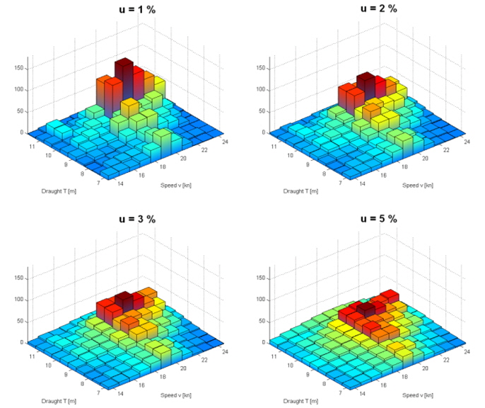
In order to represent the insecurity of the above predictions a constantly increasing, normally distributed uncertainty of 0.5% per year has been added to the respective draught and speed values. From these operations the histogram given in Fig. 8 arises.
Despite the fact, that the whole profile has been flattened, it can be seen, that the major peak originally located at T = 10.5
It has to be noted, that the chosen uncertainty can be considered to be very small value when it comes to economic predictions, but as it can be seen in Fig. 9, higher uncertainties strongly flatten the operational profile and therefore cause problems indentifying the major peak operating conditions.
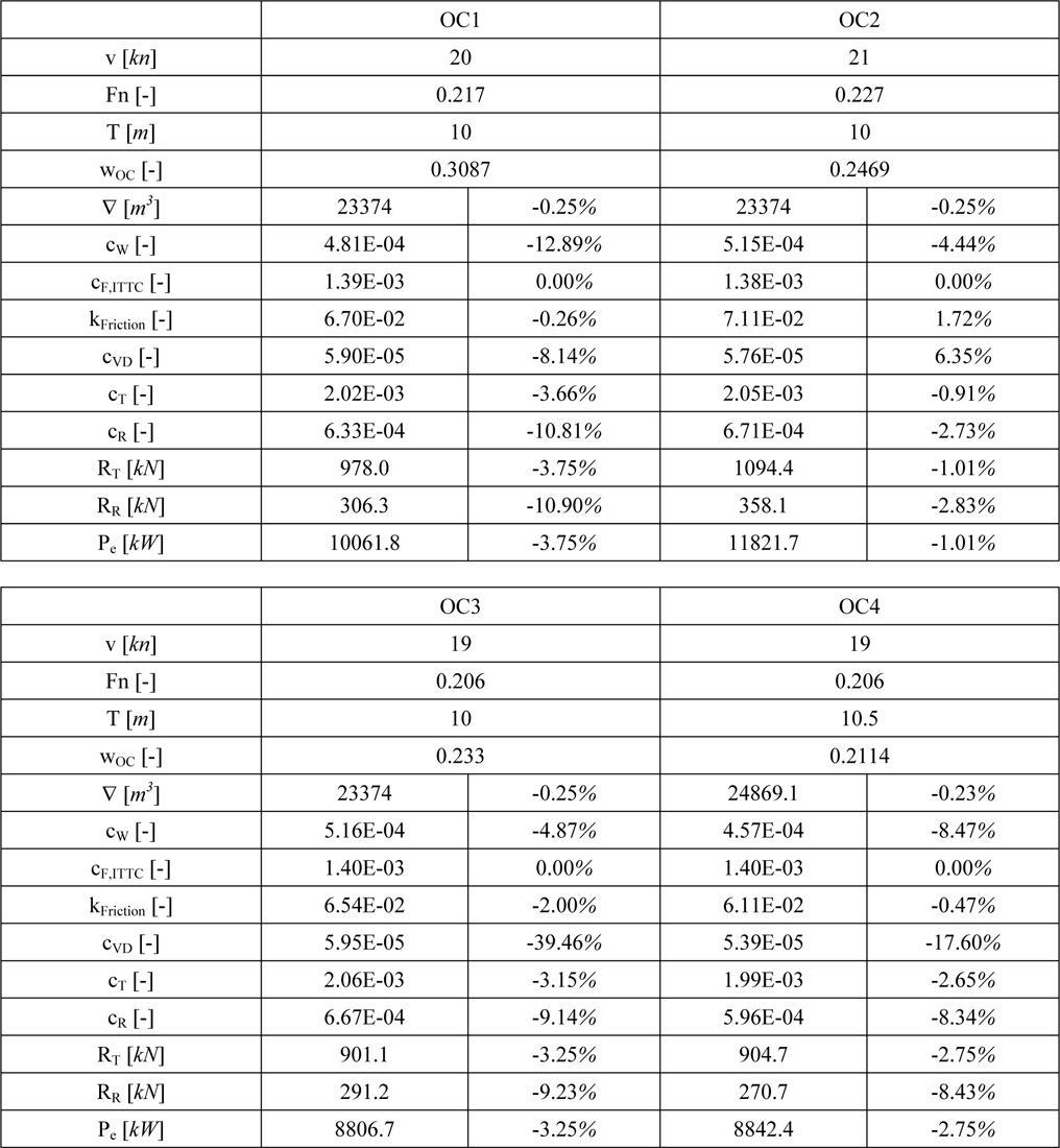
In order to derive the optimizations objective function the four major peaks covering about 20% of the vessels total operating time have been chosen to represent the KCS’ operational profile (Table 1).
[Table 1] Operational profile.
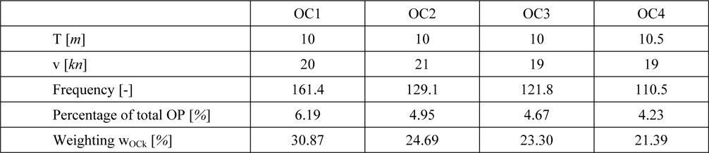
Operational profile.
The first three conditions share a draught of T = 10
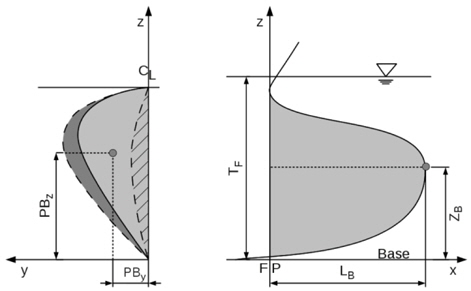
The parametric Model of the KCS is build based on the IGS-file offered by the SIMMAN 2008 workshop. Whilst the midship and the stern section have not been touched the stem has been parametrically remodeled. To do this, in compliance with Kracht (1978) the following four parameters have been introduced:
• ΔLB: change of length of bulbous bow. • ΔZB: change of height of bulbous bow. • PBy, PBz: change of breadth of bulbous bow.
The implementation of the first two parameters has been done using the
On the left side of this figure the (shaded)
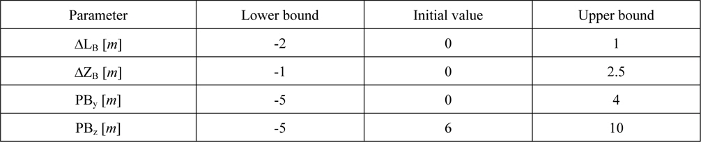
In order to define the design space the boundaries of the mentioned parameters have been chosen as follows:
[Table 2] Parameter boundaries.

Parameter boundaries.
Those values reflect the idea, that the bulbous bow should neither emerge the prow nor pierce the waterline. In case of PBy and PBz the chosen boundaries ensure a correct resistance calculation. Using the initial values leads to the original KCS hull form.
It has to be noted that in order to verify an accurate resistance calculation, the meshing of the bulbous bow has also been done as a function of the parameters ΔLB and PBy.
The optimization of the KCS’ stem section has been done with respect to the vessels weighted effective Power PE,w which is calculated for all four operating conditions by the help of the potential flow code

Here cR is the residual resistance coefficient, cF,ITTC the frictional resistance coefficient due to ITTC 57, while cVD is the viscous drag coefficient, which is an estimation of the viscous drag forces acting on the aft body of the hull form due to the thicker boundary layer. It is calculated by determining the fraction of resistance due to the viscous pressure while taking into account the maximum cp on the aft body. cW is the wave resistance coefficient and kFriction a ν-SHALLO internal form factor accounting for the change in the wetted surface area and the inhomogeneous velocity distribution (Marzi et al., 2010).
The weighted effective power then results from Eq. (2).

Thereby RT,OCk is the total resistance, vOCk the speed and wOCk the weighting of the respective operating conditions.
In a first step a
The final optimization of the five chosen starting variants has been done using the
The optimization leads to a design variant with the parameters given in Table 3.
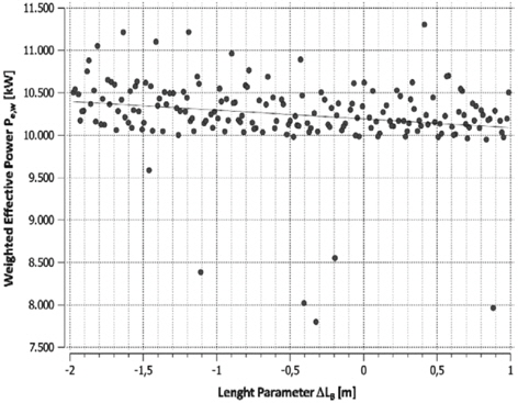
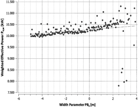
Those values acknowledge the trends gained from the
[Table 3] Optimal design parameters.
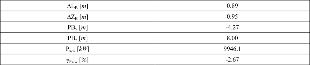
Optimal design parameters.
[Table 4] Detailed optimization results and comparison to initial hull form.

Detailed optimization results and comparison to initial hull form.
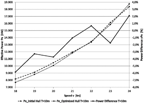
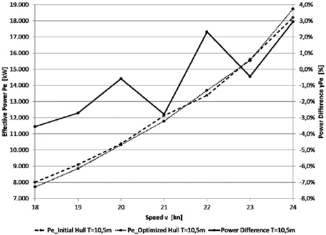
The detailed results presented in Table 4 show decreasing power values for all four operating conditions. The biggest reduction of 3.75% is achieved in OC1, mainly caused by the decreased wave resistance coefficient (-12.89%). This seems to be reasonable due to the higher weighting of this operating condition. In OC2 the smallest reduction (-1%) is achieved. This could be an allusion to the fact, that the initial KCS hull form has been designed to operate on higher speeds. This statement is also supported by the speed-power diagrams at T = 10
The above figures furthermore indicate that the initial KCS has been designed with respect to higher draughts. A comparison between the power curves for the two draughts at speed values below 21
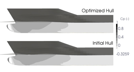
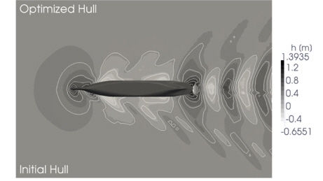
Looking closer on OC1 the comparison of the pressure distribution of the initial and the optimal bulbous bow at this operating condition (Fig. 15) as well as the respective comparison of the wave elevation (Fig. 16) give an explanation for the reduction in needed effective power.
The stagnation point at the tip of the optimized bulbous bow is smaller than its initial counterpart due to its decreased breadth. As a result of the uplifting the underpressure area at the top of the bow has become bigger leading - in conjunction with the slightly forward shifted area of overpressure - to a smaller bow wave elevation.
This effect is reflected in the comparison of the wave elevations, which shows a significant reduction within the vessels wake caused by the more advantageous wave interferences of the optimized hull form.
In general, the achieved results comply with the outcome of other related studies on the topic of hull form optimizations based on more than one operating condition. As an example Ernst and Hollenbach (2011) come to the conclusion that a multi-objective hull form optimization typically leads to reduced, less distinctive bulbous bow.
The presented method for the scenario based optimization of parametrically modeled hull forms has shown to be reliable and to achieve reductions in the needed effective power. In order to validate the method more and especially more comprehensive optimizations have to be done as the achieved results seem to be dependent on many factors.
At first, the data taken as basic input to the scenario development is of great importance. It should be taken care of, that the data cover a sufficiently long period of time and can be considered to be complete. Furthermore they should belong to a comparative vessel operating on a comparable or the same route.
The second point aims at the uncertainties. As shown in Fig. 9 the consideration of higher uncertainties results in flattened operational profiles, which leads to the need of considering more than four operation conditions within the objective function. In the course of this it should be analyzed, whether the consideration of a higher coverage of the selected operating conditions leads to better results.
Despite those factors there are some other possibilities for increasing the approaches accuracy. One exists in reducing the bins, allowing it to optimize onto more specific operating conditions. On the other hand and in accordance to the increase of uncertainties reduced bins would raise the need for considering a higher number of operating conditions in order to achieve a certain coverage. It has to be noted, that not only the size but also the bins’ position has a notable influence on the objective function.
Other possible improvements can be done by using RANSE instead of potential flow code or a more sophisticated model with more parameters that make it possible to control the complete hull form instead of only the bulbous bow.
The next steps in developing the scenario based optimization approach primarily focus on the implementation of more features into the scenario development. As an example future versions should be able to predict and consider weather conditions and should come with an enhanced objective function. The latter will be capable of executing life-cycle analyses taking into account economic parameters like for example constantly developing fuel oil prices.