The Amon-Ra instrument is the main optical payload of the proposed EARTHSHINE satellite. It consists of a visible wavelength instrument and an IR energy channel instrument to measure a global Earth albedo. We report a new sensitivity technique for efficient alignment of the visible channel instrument. Whilst the sensitivity table method has been widely used in the alignment process, the straightforward application of the method tends to produce slow process convergence because of shop floor alignment practice uncertainties. We investigated the error sources commonly associated with alignment practices and used them when estimating the Zernike polynomial coefficients. Aided with single center field wavefront error (WFE) measurements and their corresponding Zernike polynomial coefficients, the method involves the construction and use of an experimental, instead of simulated, sensitivity table to be used for alignment state estimations. A trial alignment experiment for the Amon Ra optical system was performed and the results show that 71.28 nm in rms WFE was achieved only after two alignment iterations. This tends to demonstrate its superior performance to the conventional method.
The Albedo Monitor and Radiometer (Amon-Ra) instrument is the primary payload of the proposed EARTHSun-Heliosphere Interactions Experiment (EARTHSHINE) satellite (Park et al. 2007, Lee et al 2005a, 2005b). The goal of the instrument is to measure the Earth albedo variation. The instrument consists of two optical systems. The first is a visible channel instrument to observe both the Earth and Sun alternately over the wavelength range of 0.4 ~ 0.75 μm. The other is an energy channel for bolometric measurement of the incident solar and Earth reflected shortwave radiations over 0.4 ~ 4.0 μm in wavelength. The observation concept of Amon-Ra is such that it is designed to share the same optical train as much as possible, when viewing the Earth and Sun as the spacecraft rotates (Park et al. 2007, Lee et al 2005a, 2005b). Therefore, the accurate alignment of the instrument optical system is crucial for achieving the science goal. We studied the precision optical alignment of the Amon-Ra visible channel system and report the new sensitivity table alignment technique and its alignment performance in this paper.
Over the past few decades, several computer aided alignment (CAA) methods based on the Zernike polynomials have been developed to ensure the efficient alignment of optical systems (Jeong et al. 1987, Rimmer 1990, Chapman & Sweeney 1998, Zhang et al. 2000, Kim et al. 2007, Lee et al 2007). Among them, the sensitivity table technique is arguably the most widely used method to align two-mirror and threemirror systems (Jeong et al. 1987, Rimmer 1990, Chapman & Sweeney 1998, Zhang et al. 2000, Kim et al. 2007, Bin et al. 2010, Kea et al. 2008, Zhao et al. 2010, Kim et al. 2005, Yang et al. 2004).
The technique uses Eq. 1, where [
Typically, Eq. 2 is required to build a sensitivity table (
However, it is well known that resulting
In this paper, we improve the technique with a simple and practical conceptual shift to the use of experimental sensitivity table, being away from the simulated one. Section 2 describes the theoretical method, the target optical system characteristics used and the application of the new experimental sensitivity table method. Alignment simulations and experimental results are described in Section 3, demonstrating its superior performance to that of the conventional method. In Section 4, the implications of the new experimental sensitivity method are summarized.
2. NEW EXPERIMENTAL SENSITIVITY METHOD
The experimental sensitivity table can be constructed by replacing the simulated
Once it has been built, solving Eq.1 requires for an inverse matrix
2.2 Target optical system: Two-mirror system with high obscuration
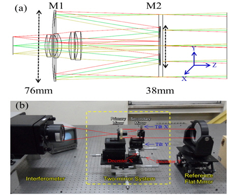
To experimentally verify the performance increase resulting from such a simple yet practical conceptual shift, we used a catadioptric optical system of high obscuration from the relatively large secondary mirror of 38 mm in diameter as shown in Table 1. Its optical system consists of two mirrors and four corrector lenses. Incident light rays are reflected from the system’s primary mirror (M1) that is 76 mm in diameter and −1.0 in conic constant, and then from its secondary mirror (M2). The M2 alignment tolerance was computed to ± 140.0 μm in decenter and ± 100.0 arcsec in tilt (Fig. 1-(a)). The system alignment was required to meet the requirement of 126.56 nm in rms WFE (Lee et al. 2005b). The alignment test configuration has the target optical system sandwiched in between a phase-shifting interferometer and a reference flat mirror, as shown in Fig. 1. M1 and the corrector lens barrel were already aligned and fixed to each other via the M1 support plate within the predetermined tolerance level. The despace between M1 and M2 was also aligned for the minimum spherical aberration value so that it was not regarded as the alignment parameter that can affected by the lens barrel states. M2 decenter and tilt are the two alignment variables that need to be controlled in order to achieve alignment, and this paper is focusing at the M2 precise alignment.
[Table 1.] Measured specification of optical elements of target optical system (Park et al. 2007).
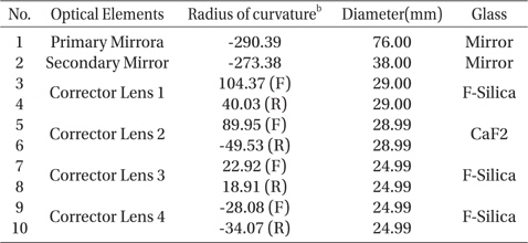
Measured specification of optical elements of target optical system (Park et al. 2007).
2.3 Simulations and experiments with experimental sensitivity table method
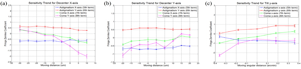
First, the experimental sensitivity table was constructed from a series of wavefront measurement at the center field. From the approximated alignment status, M2 was moved 5 μm for decenter and 0.18 arcmin for tilt in a sampling step. The system WFE was then measured, and its corresponding Zernike polynomial coefficients were obtained three times at each measurement location for decenter and tilt for x and y axes, respectively. The resulting Zernike coefficient variation trends for the y-axis tilt are shown in Fig. 2 as an example.
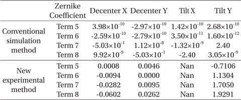
Once all the measurements were completed, we then polynomial-fit the Zernike coefficient variation over the decenter and tilt ranges used. In the polynomial fitting, we used the linear fitting equation which is the same process with Eq. 1. and 2. The final sensitivity table was then constructed, as shown in Table 2 where the resulting sensitivities from both conventional and experimental methods are compared. We note that the experiment to determine Zernike coefficients for x axis tilt was not performed because of the inaccurate goniometer tilt X motion caused by its unpredictable backlash characteristics.

Sensitivity table from the conventional simulation and from this experiment using M2 (i.e., on-axis center field measurement only).
The fringe Zernike coefficients from the 5th to the 8th term representing high order aberrations are listed in Table 2. In general, the 7th term Zernike coefficient is closely related to the x-axis decenter and the y-axis tilt, while the 8th term is sensitive to the y-axis decenter and the x-axis tilt. From Table 1, it is clear that the y-axis tilt plays the most significant role in the Zernike coefficients’ sensitivity.

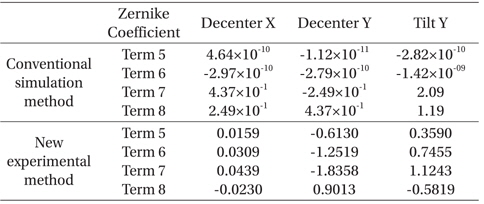
Calculated inverse matrix (A+) of using SVD technique from the sensitivity table in Table 2.
The conventional method shows ~10−10~−12 in the 5th and 6th term Zernike coefficients, illustrating the negligible effects of decenter and tilt variations on the on-axis field measurement. We note that, whilst their magnitude is somewhat smaller than the others, the 7th and 8th term coefficients also show increasing sensitivity trends similar to those of the 5th and 6th terms as well. These prove that the aforementioned measurement field positioning and apparatus control error significantly influence the resulting sensitivities.
Second, using the sensitivities in Table 2 and Eq. 4, we computed and compared the inverse sensitivity tables (
3. ALIGNMENT SIMULATION AND EXPERIMENT RESULTS
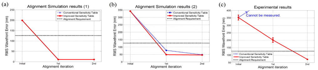
Fig. 3 shows the results from two alignment simulations and one experiment. Fig. 3-(a) illustrates the results from using the target optical system design without any additional errors included. We note that, in this ideal case, both conventional and experimental sensitivity methods are capable of producing the alignment state estimation (i.e., solution) after the first iteration.
The results in Fig. 3-(b) were obtained with 82.264 nm rms WFE in surface fabrication error introduced to M2. Both methods show similar performance in decreasing the simulated system wavefront below the requirement, although the experimental sensitivity method shows marginally better estimation after the 1st iteration.
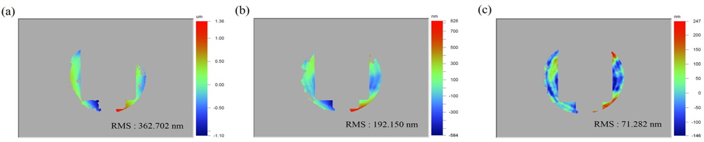
The results of the real alignment experiment appear in Fig. 3-(c). The conventional method shows an alignment divergence, even for the 1st alignment correction, which was caused by an incorrect estimation of Zernike fringe coefficients. On the other hand, the experimental sensitivity table method estimated the alignment state accurately and is capable of reducing the system’s wavefront to make it lower than the requirement in just two iterative alignment actions.
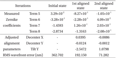
In Fig. 4 and Table 4, he initial alignment state at the center field is 362.71 nm rms WFE, where the new method’s estimate for the system’s misalignment is 0.0395 mm in the x-axis decenter, −0.0124 mm in the y-axis decenter, and −2.5472 arcmin in the y-axis tilt parameter. We adjusted the M2 location by the same amounts but to the opposite direction from the misalignment computed above. Then the alignment state improved to 192.15 nm rms WFE. After iterating one more similar alignment action with using Table 4, the optical system rms WFE became 71.28 nm in the onaxis field, excluding the masked area, which is better than the requirement, as shown in Fig. 4.
[Table 4.] The measurement results of alignment state using the experimental sensitivity table.

The measurement results of alignment state using the experimental sensitivity table.
We performed the alignment experiment for the visible channel optical system of Amon-Ra instrument successfully using the new experimental sensitivity table method. The resulting optical alignment performances between the conventional and the new technique are compared. In summary, the target optical system has technical difficulty when measuring a wavefront map because of the high obscuration (of 79.40%) caused by M2 (Park et al. 2007) and the support structure. The conventional (i.e., simulated sensitivity from the optical design) method produces an incorrect estimation of its alignment state in real experiments, largely due to the measurement uncertainties. On the other hand, the new and improved (i.e., experimentally obtained sensitivity with the on-axis center field measurement) method is capable of satisfying the WFE requirement in just two alignment actions. This proves that the experimental sensitivity method studied here would offer considerable efficiency and accuracy to the shop floor alignment process with its simplicity and high degree of practicality.