In HOS-based methods, because the performance index as the optimization criterion is nonlinear with respect to estimation parameters and these methods require a large amount of data samples. These methods have the disadvantage that their computational complexity may be large. See, for example, [1] and references therein. Since the seminal work by Tong et al. the problem of estimating the channel response of multiple FIR channel driven by an unknown input symbol has interested many researchers in signal processing and communication fields. This is achieved by exploiting assumed cyclostationary properties, induced by oversampling or antenna array at the receiver part[1,2]. The basic blind channel identification problem involves a channel model where only the observation signal is available for processing in the identification channel. Earlier blind channel identification approaches mostly depend on higher order statistics (HOS), because the second order statistics (SOS) does not contain phase information for stationary signal[3-4]. Most communication channels are time-varying in practice. Therefore, the algorithms should be able to track the change of the channel impulse response. Moreover, in a fast fading channel, the multipath channels in wireless communications vary rapidly, and we only have a few data samples corresponding to the same channel characteristics. Blind channel identification technique has been developed in adaptive algorithm based on vector-correlation method [8,9,11]. But most algorithms neglected the effect of channel noise.

Most notations are standard: vectors and matrices are boldface small and capital letters, respectively; the matrix transpose, the complex conjugate, the Hermitian, and convolution are denoted by (·)^T, (·)^*, (·)^H and ⊗, respectively; I_P is the P × P identity matrix; E(·) is the statistical expectation.

This paper is organized as follows. In section II, we review the basic assumption and identification issues. And the existing adaptive algorithms of the block LS methods are described also. A novel blind channel identification technique based on eigenvlaue decomposition and adaptive implementation are proposed in section III. Simulation results with real measured channel are performed in section IV. Section V concludes our results.

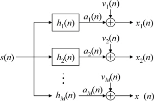
In this paper, consider a special case, when the channel output is two times oversampled or there are two antennas at the receiver, this is equivalent to two channel representation (M=2). From the Fig. 1, in the absence of noise, it is apparent that the output of each subchannel is

Then

Let 𝒳(t) be the signal at the output of a noisy channel

where s(k) denotes the transmitted symbol at time kT , h(t) denotes the continuous-time channel impulse response, and v(t) is additive noise. As shown in [3], the single channel system can be considered as the multichannel system by the sampling the received signal at a rate faster than the input symbol rate. The source signal s(n) then passes through M equivalent symbol rate linear filters. And as shown in Fig. 2, x_i(n) denotes the output from the ith channel with the noisy FIR channel impulse response {h_i(n)}, which is driven by the same input s(n). Clearly, for linearly modulated communication signals, x_i(n) , a_i(n) , s(n) , v_i(n) , and h_i(n) are related as follows

where L is the maximum order of the M channels.

The blind identification problem can be stated as follows: Given the observation of channel output {x_i(n) , i=1,⋯,M; n=L,⋯,N}, determine the channels and further recover the input signals {s(n) }. As in classical system identification problems, certain conditions about the channel and the source must be satisfied to ensured identifiability. We assume the following throughout in this paper about the channel and source conditions.

A1) Subchannels do not share common zeros, or in other words, they are coprime.A2) The noise v(n) is zero mean, white with known covariance, no cochannel correlation, and uncorrelated with source signal.A3) The channel has known order L.

The assumption that L is known may be practical. To address this problem, there are three approaches[5]. First, channel order detection and parameter estimation can be performed separately. Second, some statistical subspace methods require only upper bound of L. Third, channel order detection and parameter estimation can be performed jointly.

As described in [5], to avoid the trivial solution to minimization problem a proper condition must be selected. In this section, a new approach is proposed that is based on eigenvalue decomposition. Indeed, the eigenvector corresponding to the minimum eigenvalue of the covariance matrix of the received signals contains the channel impulse response. This approach is based on the unit norm constraint that is apart from the linear constraint introduced in the previous section[6].

Number equations consecutively with equation numbers in parentheses flush with the right margin, as in (1). We assume that the channel is linear and time invariant within small time interval; therefore, we have the following relation as described in (4)

where

and the channel impulse response vector of length L are defined as

The covariance matrix of the two received signals is given by

Consider the 2L´1 vector as follows:

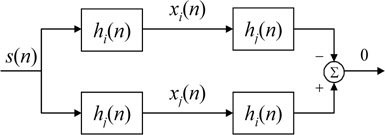
From (5) and (8), it can be seen that R_xh=0, which means that the vector h is the eigenvector of the covariance matrix R_x corresponding to the eigenvalue 0.

Moreover, if the two channel impulse response h₁ and h₂ have no common zeros and the autocorrelation matrix of the source signal s(n) is full rank, which is assumed in the rest of this paper, the covariance matrix R_x has one and only one eigenvalue equal to zero. Consider the noisy channel case as described in (2) and let M=2. It follows from (1) that

where x(n)=[x₁^T(n)) x₂^T(n)]^T and v(n)=[v₁^T(n)) v₂^T(n)]^T .

If the correlation matrix of the vector x(n) is denoted by R_x, a direct of conclusion of (10) will be

We note from (11) that h is the eigenvector of the correlation matrix R_x and is the corresponding eigenvector of R_x. The knowledge of can be obtained as a by product if wanted.

In practice, it is simple to estimate iteratively the eigenvector corresponding to the minimum eigenvalue of R_x, by using an algorithm similar to the Frost algorithm that is a simple constrained LMS algorithm [7].

Minimizing the quantity h^HR_xh with respect to h and subject to ∥h∥²=h^Hh=1 will give us the optimum weight h_opt.

Let us define the error signal

where x(n)=[x₁^T(n)x₂^T(n)]^T . Note that minimizing the mean square value of e(n) is equivalent to solving the above eigenvalue problem. Taking the gradient of e(n) with respect to h(n) gives

and we obtain the gradient-descent constrained LMS algorithm:

where μ, the adaptation step-size, is a positive constant. Substituting (13) and (14) into (15) gives

and taking statistical expectation after convergence, we get

which is what is desired: the eigenvector h(∞) corresponding to the smallest eigenvalue E[|e(n)|²] of the covariance matrix R_x.

In practice, it is advantageous to use the following adaptation scheme

The algorithm (18) presented above is very general to find the eigenvector corresponding to the smallest eigenvalue of any matrix R_x. If the smallest eigenvalue is equal to zero, which is the case here, the algorithm can be simplified as follows:

and

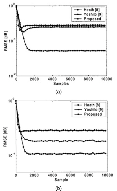
Computer simulations were conducted to evaluate the performance of the proposed algorithm in comparison with existing algorithms. In all the simulations, two channel SIMO model is assumed. This means two times oversampling or two sensors at the receiver in real situation. The input signal is 4-QAM. For simplicity of comparison, we assumed that the channel order Lis known. The performance index is achieved by examination the root mean square error (RMSE) that is defined as [4].

where N_t is number of Monte Carlo trials, and is the estimate of the channels from the ith trial.

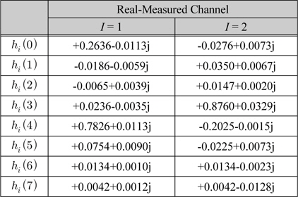
We used real-measured microwave channel. The shortened length-16 version of an empirically measured T/2-spaced digital microwave radio channel ( M=2) with 230 taps, which we truncated to obtain a channel with L=7. The Microwave channel chan1.mat is founded at http://spib.rice.edu/spib/ microwave.html.

The shortened version is derived by linear decimation of the FFT of the full-length T/2-spaced impulse response and taking the IFFT of the decimated version (see [10] for more details on this channel). The channel coefficients for both sets of channels are listed in Table 1. A total number of 50 independent trials were performed. All algorithms were initiated at h(0)=[1, 0, ..., 0, 1, 0, ..., 0]^T with the step size μ=0.01.

Fig. 3 shows the RMSE of the channel estimates from existing algorithms and the proposed algorithm. From these figures, we can see that the proposed algorithm always performs better than others. By inspection, we can observe that RMSE values of the proposed method are decreased more or less 6-10 dB, and 1-2 dB under 20 dB, and 10 dB, respectively. Clearly, we can observe the significant improvement of the proposed algorithm over existing algorithms.

In this paper, an approach to channel identification has been presented. The method is based on eigenvalue decomposition. The eigenvector corresponding to the minimum eigenvalue of the covariance matrix of the received signals contains the channel impulse response. And we use a simple constrained LMS algorithm to estimate iteratively the eigenvector corresponding to the minimum eigenvalue. In comparison with algorithms, the proposed one seems to be more efficient in a low SNR channel and much more accurate.