Dynamic Positioning (DP) is an automatic position control system using propellers or thrusters for offshore floating structures. Recently, the maritime operation area has expanded into the deep sea. Because a mooring system is not economically feasible in the deep sea, DP has been studied more than ever before, by many research groups. In particular, ocean prospectors, like drilling rigs or drill ships, have to move around in an oilfield development zone, so a DP capability analysis is performed in the basic design stage of these vessels.
The position and velocity vectors of a DP vessel are measured by the Differential Global Positioning system (DGPS) / Inertial Navigation System (INS) in real time. The measured position and velocity vectors contain measurement noise and process noise. The main process noise can be regarded as environmental disturbances that threaten the survivability of a structure, and interfere with its stable operation. Thus, disturbances are an important matter, which must be taken into consideration. But the most common DP control system has a simple linear controller, combined with a wind feedforward controller, in which there is no consideration of other disturbances (ocean current or wave load). Moreover, because the wind feedforward controller is designed based on experimental data or empirical regression formula, it may not be possible to compensate for the wind load exactly. It is hard to estimate and to compensate for ocean environmental disturbances in real time, so the control system has to be designed with consideration of not just the dynamical characteristics of an ocean structure, but also unknown ocean disturbances.
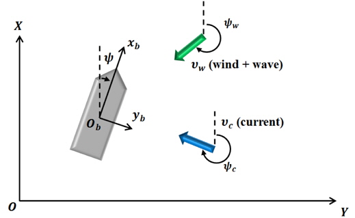
Weather-vaning is to make the heading angle of a DP vessel head towards (or away from) for the disturbance direction. Most ocean floating structures have long longitudinal length. So the disturbance incoming in the transverse direction of a DP vessel induces larger force and moment, compared with the longitudinal direction. Weather-vaning enables a DP vessel to maintain its position with minimum control force through matching the heading angle of a DP vessel with the disturbance direction.
In this paper, an auto weather-vaning system for a DP vessel using a nonlinear controller and disturbance observer is proposed. It is almost impossible to measure the exact force and moment induced by ocean environmental disturbances (the ocean current, wave and wind) in real time. It can be called the disturbance uncertainty, which degrades the performance of a designed controller. Generally, a controller is designed by using only a plant model without disturbance, so the control performance of the closed-loop system does not have to be as good as expected. To deal with this problem, the disturbance observer is introduced. It guarantees the robustness of the closed-loop system, by transforming a real plant, into a nominal model without disturbance. The weather-vaning system continuously changes the heading angle of a DP vessel. Because of kinematic nonlinearity, a nonlinear control method is more efficient than a linear control method. This paper used a backstepping controller as the DP controller, which has already been proven for its stability and performance by several research groups.
Since the late 1990s, there have been many studies of DP controllers and observers. A mathematical model of a DP vessel was constructed, and an LQG feedback controller and a model reference feedforward controller were proposed by Sørensen (1996). A nonlinear controller for ocean structures, like a feedback linearization and backstepping, was presented (Fossen, 1994; 2002). Sørensen (2011) wrote a survey paper that contains a lot of previous research materials about DP controllers and observers. The research about a disturbance observer has been studied by electrical and mechanical field research groups (Radke and Gao, 2006; Schrijver and Dijk, 2002; Shim and Joo, 2007; Choi et al., 2003). The research about a nonlinear observer to estimate the angle of attack for a missile autopilot system in the presence of the model uncertainties (Lee et al., 2011). But the researches in which a disturbance observer is applied to the DP system have not been studied. Ocean structures are always unavoidably exposed to disturbances, so it is most appropriate to apply a disturbance observer to ocean structures. There are a few researches about weather-vaning systems. Most papers about weathervaning have focused on passive weather-vaning, which only depends on the yaw moment induced by disturbances, without any active actuator operations (Chilliamcharla et al., 2009; Morandini and Wong, 2007). The paper performs the motion analysis of a DP vessel that is free to rotate in the yaw direction. Fossen and Strand (2001) proposed Weather Optimal Positioning Control (WOPC) for a DP vessel. The methodology in that paper enables a DP vessel to minimize energy consumption, by introducing a gravity field concept into 3 DOF horizontal planes. It can be said that this is a kind of active weather-vaning system, by using actuators. But in this methodology, there is no consideration of the magnitude and frequency characteristics of disturbances. On the other hand, a disturbance observer for a weather-vaning system can be designed based on the consideration of the disturbance characteristics.
The paper is described in the following order. First of all, the mathematical model of a DP vessel is described. The mathematical model is composed of two parts. One is the low-frequency model, and the other is the wave-frequency model. In the model, the characteristics of disturbances are described. The ocean current, wind and wave are described respectively. Then, the controller and the disturbance observer are described. The basic concepts are briefly explained, and the design procedures are explained in detail. Next, a weather-vaning algorithm is explained. The effectiveness of the proposed method is validated, by the numerical simulations of a semi-submersible type vessel. Finally, the conclusion summarizes the research results.
First of all, the coordinate systems for a mathematical model are defined. The dynamic model for a DP vessel consists of two parts (Sørensen, 1996; Fossen, 2002). One is a linear wave-frequency model, and the other is a nonlinear low-frequency model. The linear wave-frequency model is about an oscillatory motion induced by a linear wave. It is zero-mean oscillatory motion that has high frequency, so it not only has bad influence on actuators, and but also belongs to uncontrollable motion. The nonlinear low-frequency model is of the slowly varying motion induced by environmental disturbances, which accounts for the ocean current, and second order wave and wind loads. This motion has low frequency, and makes a DP vessel move away from its desired position. Thus it is the motion that must be controlled for stable operation. But because the DGPS/INS measures these two motions together, the wave frequency motion is generally filtered by a low pass filter or observer system.
Two different reference frames are defined. There are the earth-fixed reference frame
If only 3 DOF horizontal motions (surge, sway and yaw) are considered, the earth-fixed position vector and the body-fixed velocity vector are given by reference frames for a DP vessel:

The 3 DOF relation between the body-fixed frame and the earth-fixed frame is as follows:

where,
The linear wave-frequency model is considered as the motion induced by irregular wave, which is the linear superposition of first order waves with different frequencies and amplitudes. It can be said that the analysis of this motion is the same as the conventional seakeeping problem (Lewis, 1989). The 6 DOF equations of motion are formulated as:

where,
>
Nonlinear low-frequency model
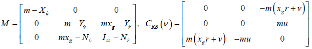
The nonlinear low-frequency model is considered as the motion induced by environmental disturbances which consist of the ocean current, second order wave and wind loads. The first order wave does not induce the drift motion, so it is not included in environmental disturbances. The analysis of this motion is similar to the conventional ship maneuvering problem (Lewis, 1989). But the model has several environmental disturbances, unlike the maneuvering problem. It is assumed that the disturbances induce only 3 DOF horizontal motions.

where,
i) The body-fixed frame is located at the principal axis frame. Ixy = Iyz = Ixz = 0 ii) The mass of the DP Vessel is distributed symmetrically to the left and right. yg = 0 iii) All hydrodynamic coefficients are constant.
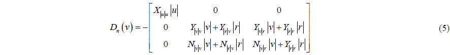
In (4), all of the matrices can be written:

τcon =[τx τy τψ]T, d = [X2nd_wave + Xwind Y2nd_wave + Ywind N2nd_wave + Nwind]T
The nonlinear part in the damping matrix

>
Ocean environmental disturbances
As previously mentioned, ocean environmental disturbances include the ocean current, and second order wave and wind loads. The force and moment by the ocean current are considered as the relative velocity between a vessel and the current velocity. The nonlinear low-frequency model is described in the body-fixed frame, so the earth-fixed current velocity vector has to be transformed to the body-fixed current velocity vector. The relationship between the two vectors is as follow:
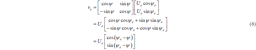
where,

The relative velocity is used in the nonlinear low-frequency model (4).
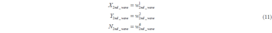
The second order wave loads is divided into mean, slowly varying loads and rapidly varying motion. It can be calculated by means of quadratic transfer functions for,

where,

By the approximations, the slowly-varying load is included in the mean drift load. Eventually, the wave drift load can be defined by dividing the wave spectrum into N equal frequency intervals with frequency

where > 0 is the frequency-dependent wave drift function, and

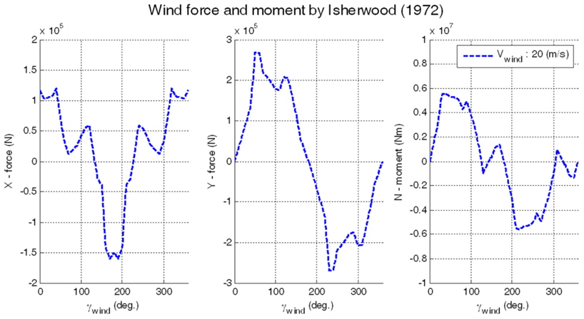
There are several regression methods to estimate the force and moment by the wind for marine structures (Blendermann, 1995; Gould, 1982; Isherwood, 1972; OCIMF, 1994). But these methods have been developed for ships. There is a research about the wind load for pontoon type floating structures (Kitamura et al., 1997). All of the estimated methods need the specific geometric information of the upper structures of a vessel. It is hard to know this exact information, so it is difficult to implement the wind load. This study assumes the wind load of a DP vessel is similar to that of other vessels with similar size. The regression parameters of Isherwood (1972) are used.
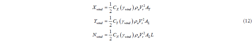
where,
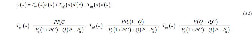
This paper proposes a nonlinear controller to control the 3 DOF horizontal (surge, sway and yaw) position vector. The nonlinear control method has the advantage of exactly dealing with a nonlinear system, but it also has the disadvantage of the difficulty of designing a controller, and analyzing its stability. On the other hand, the linear control method has been well developed by many previous studies, so that most industries have mainly used the linear control method. The DP is also no exception. Most of the DP control systems use a linear controller. However, because our eventual goal is the weather-vaning, the designed controller is capable of not only maintaining the desired position, but also changing the yaw angle of a vessel at the same time. Because of the nonlinearity of a DP vessel’s kinematics, the exact position vector cannot be expressed as a linearized rotation matrix. For this reason, a nonlinear control method is used as the DP controller, instead of a linear control method. From the 1990s, some nonlinear control methods for a DP control system have been researched. They are well documented in some books and papers (Sørensen, 2011; Fossen, 2002). Among nonlinear control methods, the backstepping control method is used in this paper. The backstepping control method was developed for nonlinear dynamical systems in the early 1990s (Kokotovic, 1992; Lozano and Brogliato, 1992). This method determines a control law through the recursive construction of a Lyapunov function candidate step-by-step. A stabilizing function and a backstepping variable are defined in each design step and the actual control input is determined in the last design step. Because each design step is affected by the immediately previous design step, the design procedure of the controller is simple. In other words, the construction of Lyapunov function candidates and the control gain selection are easy. The stability of the nonlinear closed loop system is easily verified theoretically, by using the Lyapunov stability theorem. The design process of the backstepping controller for a DP vessel is explained in reference Fossen (2002). First of all, the design goal is to make the position vector
The first backstepping variable

The time differentiation of (13) is as follows:

The velocity vector


A first Lyapunov function candidate for the

The time differentiation of (17) is as follows:

To make (18) negative about


By substituting (19) into (16) and (18), we can get


The above (22) cannot be negative, because of the second term
The second backstepping variable

To use the dynamical model of 3 DOF horizontal motions (4), multiply (23) by the inertia matrix

Because the mathematical model of a DP vessel is a second order differential system, any virtual control or backstepping variables are no longer needed, and the actual control input

By substituting (24) into the time differentiation of (25), we can get:

To make (26) negative, the actual control input

where is the estimated value of the disturbance by the disturbance observer.

By substituting (27) into (23) and (26), we can get:


If the disturbance observer eliminates the disturbance exactly, the time differentiation of the second Lyapunov function candidate can be strictly negative about the backstepping variables

By the Lyapunov Stability theorem,
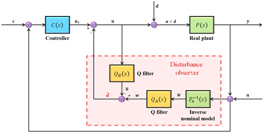
The basic concept of the disturbance observer is to use an inverse nominal model to eliminate the disturbance and modeling uncertainty. It is easy to combine a closed loop system with the disturbance observer, because it constitutes an inner-loop. The basic structure of the disturbance observer is illustrated in Fig. 2.
In Fig. 3,

If
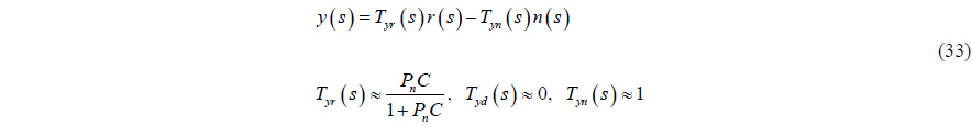
Generally, the disturbance is a low-frequency component, and noise is a high-frequency component. In the low-frequency region, the output is considered as follows:


where,
To design the disturbance observer for a DP vessel, the nominal model of a real plant is determined, and the relative degree of the nominal model is examined. First of all, the low-frequency motion (4) is linearized at the point that all states are zero.

The state space form of (4) is as follows:

The determinant of the system inertia matrix

Because is the surge added mass, it has negative sign, so (

where,
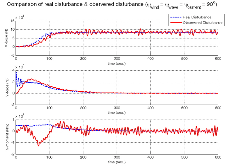
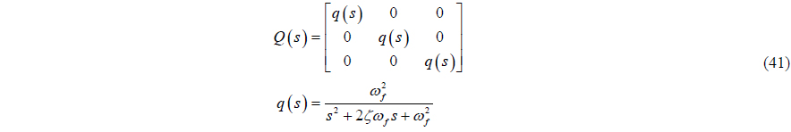
In order to estimate the disturbance

In (40), the estimated disturbance involves the ocean current, wind and wave loads. It is assumed that the 3 DOF horizontal control force and moment
Because the disturbance observer makes a real plant into a nominal model without disturbance, it can be known that the performance of the controller is more robust, than the case of using only the controller.
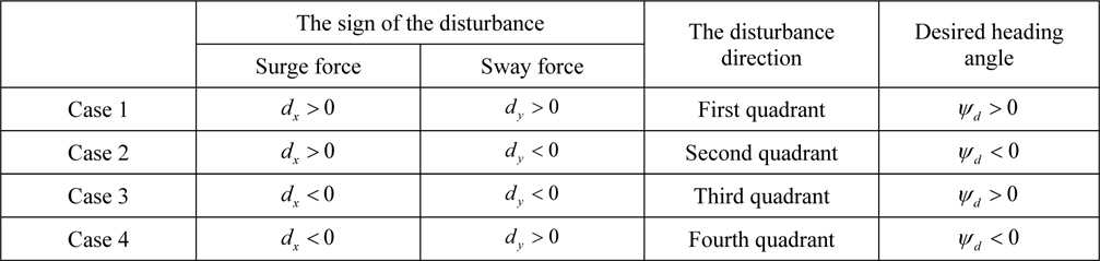
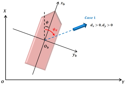
To implement the weather-vaning, the disturbance direction has to be defined. The effect of three kinds of disturbances (ocean current, wind and second order wave) is combined, and considered as a single disturbance. When the heading angle (or the opposite heading angle) of a DP vessel is matched with the direction of this single disturbance, the vessel can maintain its position with minimal control force. One can easily find out which quadrant the disturbance direction belongs to in the bodyfixed frame. The relations of the disturbance direction and command heading angle
[Table 1] The disturbance direction estimated by using the sign of the single disturbance.

The disturbance direction estimated by using the sign of the single disturbance.
Case 1 defined in Table 1 is illustrated in Fig. 3.
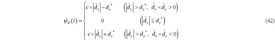
If the estimated disturbances in surge and sway axes are all positive, it can be known that the yaw angle, which minimizes the estimated disturbance in the sway axis, exists in the first quadrant in the body-fixed frame. In this case, the desired heading angle is also positive. While the desired heading angle increases, the yaw motion stops at the moment in which the estimated disturbance in the sway axis is small enough. This paper defines the criteria as

By the above relation, the desired heading angle is changed. The rate of the desired heading angle is proportional to This means that if the difference between the vessel’s heading angle and the desired heading angle is large, the desired heading angle changes rapidly; if not, it changes slowly. The constant
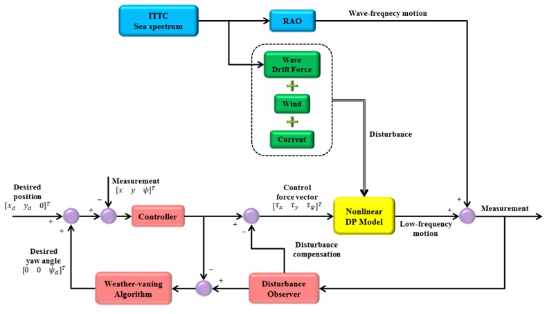
The whole flow of the numerical simulation is illustrated in Fig. 4. First of all, the wave-frequency motion is generated by using the ITTC sea spectrum and the motion RAO. The disturbances are composed of the ocean current, wind and wave drift force. The output of the nonlinear DP model enters the feedback loop and the disturbance observer. The estimated disturbance is the input of the weather-vaning algorithm to calculate the disturbance direction in real-time. The calculated disturbance direction becomes a 3 DOF horizontal reference, input with the desired position. The control input consists of the output of the controller part and the disturbance compensation part.
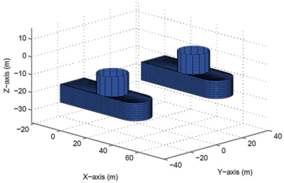
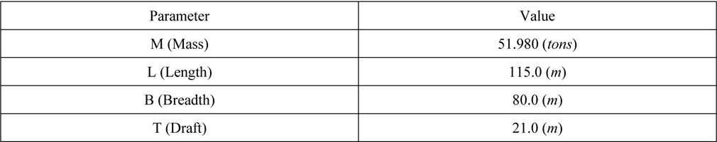
The DP vessel used for the numerical simulation is a semi-submersible type vessel. The under structure shape of the vessel is illustrated in Fig. 5. Because the shape is of front-back symmetry, only the front side shape is shown. The main dimensions are listed in Table 2.
[Table 2] Main dimensions of the semi-submersible type vessel.

Main dimensions of the semi-submersible type vessel.
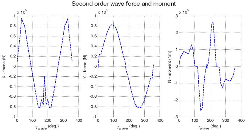
Marine Systems Simulator (MSS) Hydro is used to get the hydrodynamic forces (Perez et al., 2006). The wind load can be calculated from the specific upper structure information of the vessel. This paper assumes the wind load of the semi-submersible vessel is similar to that of a general ship. The wind and wave loads used are illustrated in Figs. 6 and 7.
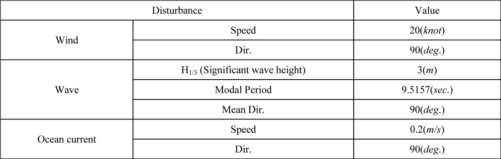
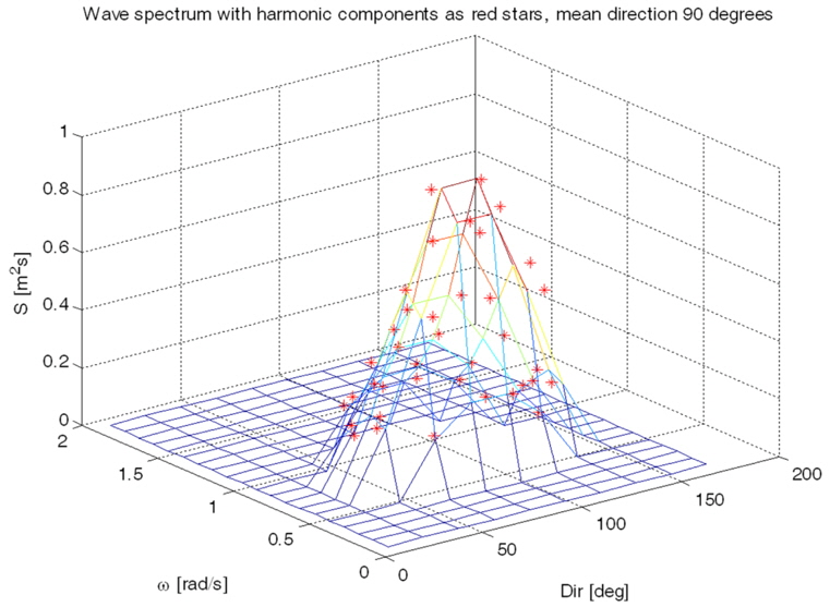
The disturbance condition is listed in Table 3. The wind speed and direction, the significant wave height and mean direction, and the ocean current speed and direction are presented. In Fig. 8, ITTC wave spectrum is illustrated. The spectrum is short-crested wave spectrum which has one modal point. In real world, the spectrum may have two or more modal points, so it can not reflect the actual wave condition. But, the focus of this paper is disturbance rejection and weather-vaning. The number of modal points does not affect the performance of proposed controller and disturbance observer because the cut-off frequency of the disturbance observer has to be determined by the frequency bandwidth of ocean disturbances. Thus, it does not matter which shape of spectrum is used. In order to check the performance with the most extreme conditions, all disturbance directions are 90°.
[Table 3] Disturbance conditions.

Disturbance conditions.
Actually, the control force vector has to be allocated actuators like propellers or thrusters, which are installed on the DP vessel. This is another problem, which is called the control allocation. In particular, most semi-submersible type vessels have azimuth thrusters that have two degree movement freedom (azimuth angle, and thrust). This is a nonlinear control allocation problem, which is not covered in this paper. Instead, in order to consider indirectly the effect of actuators, first order systems are used, as follows:

where,

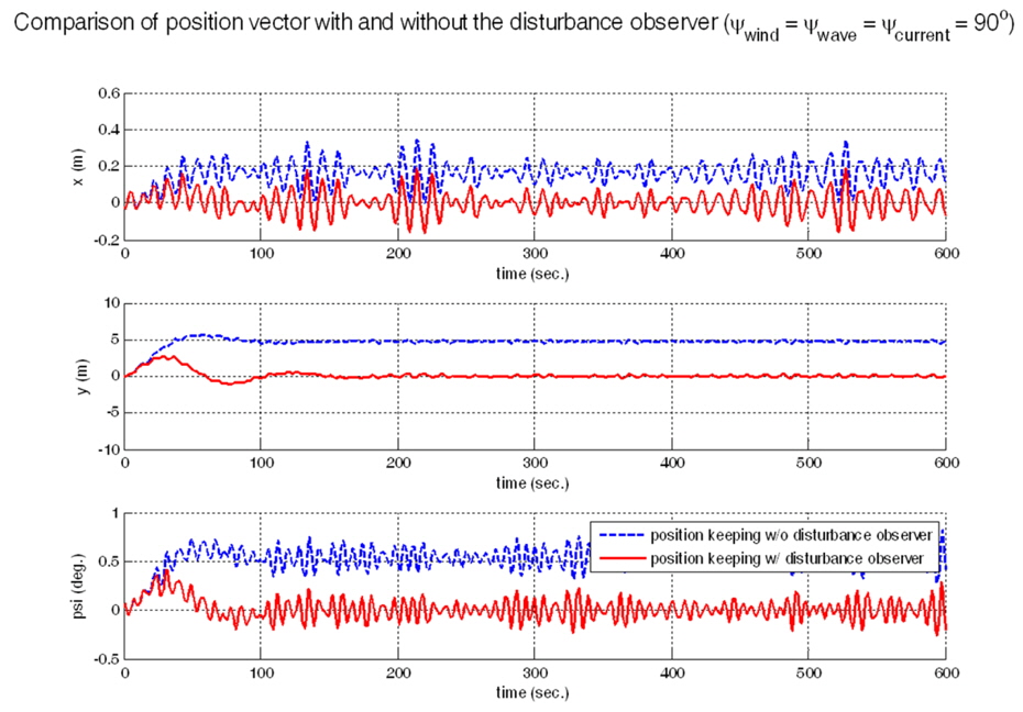
The time responses of the position vector and the control force vector are shown in Figs. 7 and 8. The simulation time is 600 seconds. To show robustness of disturbance observer based controller, simulations are performed about the case using only controller and the other case using not controller but disturbance observer. The simulation results are in Fig. 9. In the case of no disturbance rejection by disturbance observer, there is steady state error compared with the case with disturbance rejection, although the control gain matrix is the same.
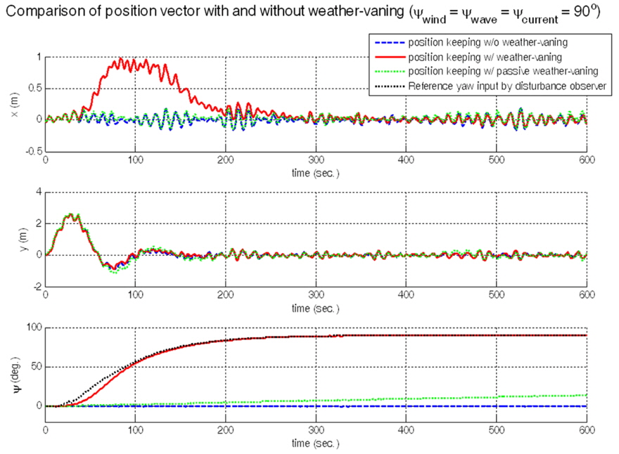
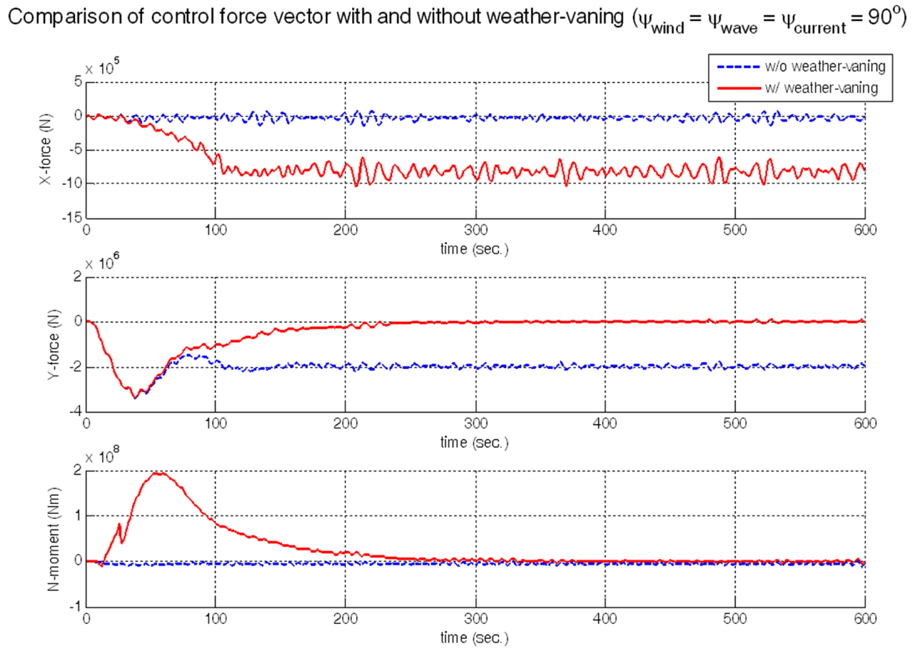
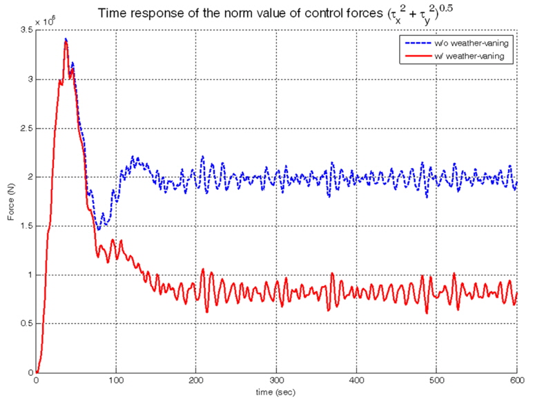
The other simulation is about comparison according to the presence of weather-vaning. The simulation results in Figs. 10 and 11. In Fig. 10, it seems that the case of not using weather-vaning is more efficient for position keeping than the case of using weather-vaning. But the position error is less than 1
After about 80
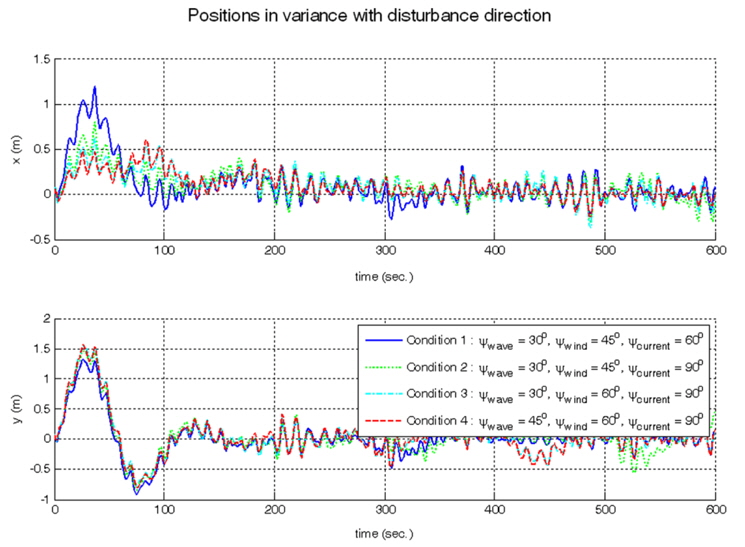
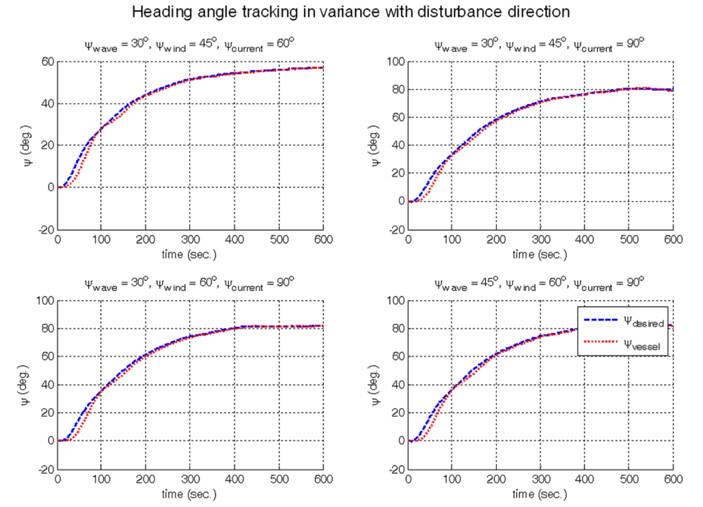
To verify proposed method in various direction of disturbances sea conditions, simulations are performed in the combination of the four kinds of disturbance directions.
[Table 4] Disturbance conditions.
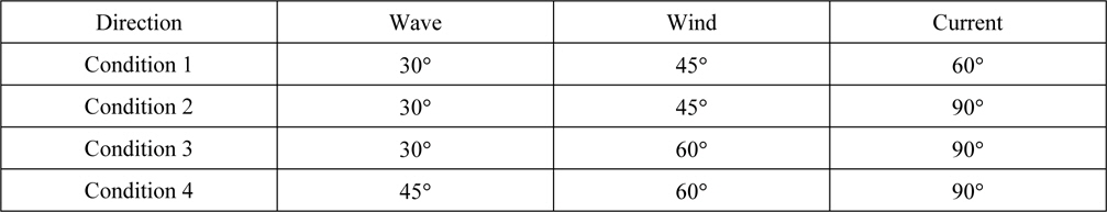
Disturbance conditions.
In Fig. 14 and in Fig. 15, although the directions of disturbance are not the same and different each other, it is shown that the position keeping and the heading angle tracking are well performed.
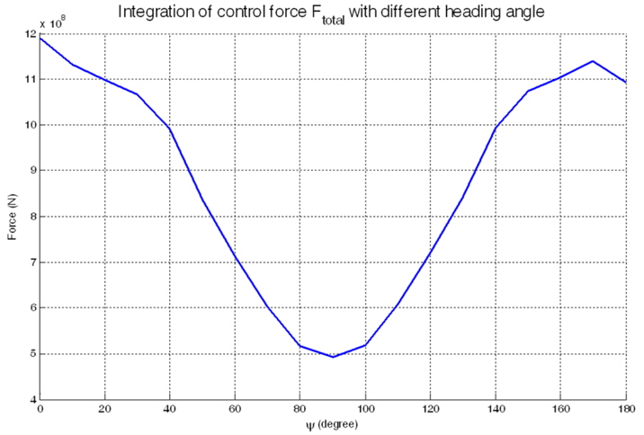
To check whether the weather-vaning algorithm enables the control forces to minimize or not, the integration of control force with heading angle of the DP vessel from 0° to 180° with interval degrees 10° is performed.

The comparison results is in Fig. 14.
In Fig. 14, the minimum point appears at about a heading angle 90°. This is a reasonable result in the consideration of the disturbance conditions of Table 3. By this, the proposed weather-vaning system enables the DP vessel to keep its position, with the minimum control force. Thus it can be known that the ocean operations are performed in not only a stable but also an economically efficient condition.
The paper presents an auto weather-vaning system for a DP vessel. The mathematical model of a DP vessel is constructed. The model is divided into two parts, the wave-frequency model and the low-frequency model. The kinds of disturbances (ocean current, wave and wind) are described. The disturbance observer is designed to eliminate the effect of ocean disturbances, and to estimate the disturbance direction. The backstepping controller is designed to not only maintain the position, but also to implement the weather-vaning algorithm. The weather-vaning algorithm can determine the disturbance direction by using the estimated disturbance, which is the output of the disturbance observer in real time. Finally, two numerical simulations are performed for a semi-submersible type vessel. The one is about disturbance rejection performance by comparison of the presence of disturbance observer. The other is about weather-vaning performance by comparison of the presence of weather-vaning algorithm. The results show that the proposed method make a DP vessel maintain its position with the minimum control force.