Sea loads considerably influence on offshore structures’ safety, safety for workers, and efficiency of work in the ocean. Sea loads are the major influencing factors that have to be carefully considered when the structures are in operation. Many studies on sea loads are in progress. Especially, wave induced loads are the dominant factors to be considered. In order to estimate the wave induced loads, the accurate prediction of wave itself is critical.
In order to predict accurate wave field around offshore structure, the mechanism of wave propagation should be established. Wave propagation prediction has many practical applications. Just name a few of them, prediction of wave near floating structures are necessary for the safe operation of the structures. We can get benefited from estimating the safe time period for landing of helicopters on offshore structures or on warships. The damage caused by sloshing can be avoided if one can estimate the sloshing load from wave prediction by taking countermeasures.
At present, the usual practice of wave measurement is using wave gauge at a fixed point. Using the linear wave theory and the principle of superposition, the integral equation can be derived from the time series data at the fixed point. The generated integral equation is called Fredholm integral equation of the first kind. With integral equation discretized by wave number and time, the equation which relates wave amplitude and wave spectrum can be formulated. Wave amplitude spectrum can be obtained by solving the constructed matrix and using wave amplitude spectrum. Wave elevation at arbitrary points and time can be estimated. The discretized integral equation is mostly ill-conditioned which leads to unstable solutions. In order to estimate accurate wave elevation at target point, Tikhonov regularization method is introduced (Fridman, 1956; Isakov, 1998; Kammerer and Nashed, 1972; Tikhonov, 1963). When it comes to the Tikhonov regularization method, choosing optimized regularization parameter is essential to ensure the stability and accuracy of matrix. Present study employed the L-curve method.
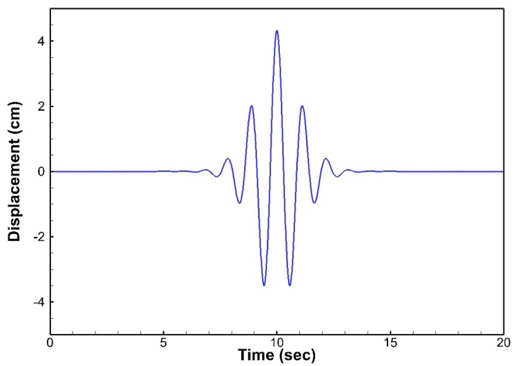
In this study, Gaussian wave packet is introduced to realize the incoming waves. Numerical simulation of the Gaussian wave has been conducted. The accuracy was evaluated by performing numerical and analytic works on this. Furthermore, the wave propagation experiment in wave tank is conducted. The wave time series has been measured at a fixed point. By analyzing the data, the wave field at the target point is estimated. Again, the ill-posed system is solved by applying Tikhonnov regularization method. The regularization parameter was estimated by the L-curve criterion which was successfully introduced by Lawson and Hansen (1974). The estimated wave time series was compared with the measured time series. The present scheme can be extended to multidirectional short crested sea if a spreading function is introduced. The present study is limited to linear dispersive waves due to its mathematical formulation. Therefore one should come up with non-dispersive scheme to deal with nonlinear wave field.
Assuming an ideal fluid, with its motion irrotational for a small amplitude wave, the wave elevation can be written as

where

where

where
>
A fredholm integral equation of the first kind; ill-posed problem
Eq. (2) is a Fredholm integral equation of the first kind. The wave elevation shown in the left hand side of the Eq. (2) will be a given function from measurement. The term
If the given problem is not well-posed, it is said to be ill-posed. Therefore the problem we have formulated is an ill-posed problem. The remedy for the ill-posed problem is regularization which will be covered in a latter chapter. If we discretize the Eq. (2) the matrix we encounter becomes ill-conditioned matrix.
>
Discretization of the integral equation
A typical and most often used method of approximating an integral is first to discretize the integrand given in a continuous function into a finite number of segments and then the original integral is reduced to a sum of the integrals of the segments. Then the wave elevation in Eq. (2) can be approximated by

where
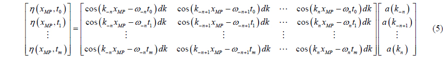
Rewriting the above equation as :

where

where
[Table 1] Simulation parameters.
Simulation parameters.
REGULARIZATION OF WAVE PROPAGATION MODEL
Before solving Eq. (6), the stability of matrix has to be examined. In order to verify the stability, condition number of the matrix should be checked. By singular value decomposition, matrix

where
The condition number of matrix

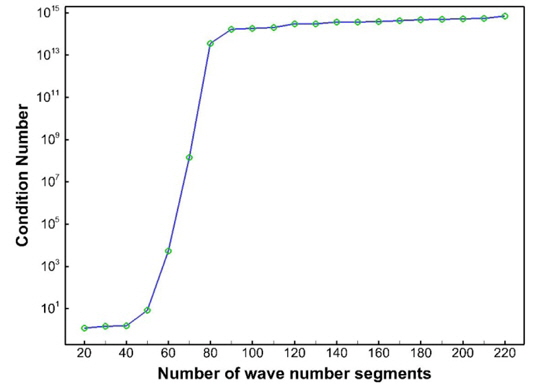
The matrix which has a small condition number is called a well-conditioned matrix. However, the matrix with a large condition number is called an ill-conditioned matrix which is hard to acquire stable solution. Fig. 3 shows the condition number of the kernel of the Eq. (6) for various number of wave number segments. As shown in Fig. 3, the matrix turned into ill-condition as the number of segments is increased. The small number of segments helps the stability of the matrix. On the other hand, the number of segments has to be increased to describe wave information more accurately. A method has to be introduced to increase the number of segments and stabilize the matrix simultaneously.
>
Regularization of wave propagation model
By using least square method, the amplitude spectrum and wave elevation can be expressed as:

where

where
Choosing an appropriate regularization parameter is crucial in obtaining a stable solution when Tikhonov regularization method is used. The success of the regularization depends on a proper choice of the regularization parameter


Also,

Substituting


where

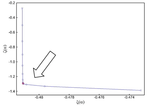
By using the L-curve method, the desired regularization parameter is obtained from the point of maximum curvature in the L-curve and this point is marked in red circle in Fig. 4.
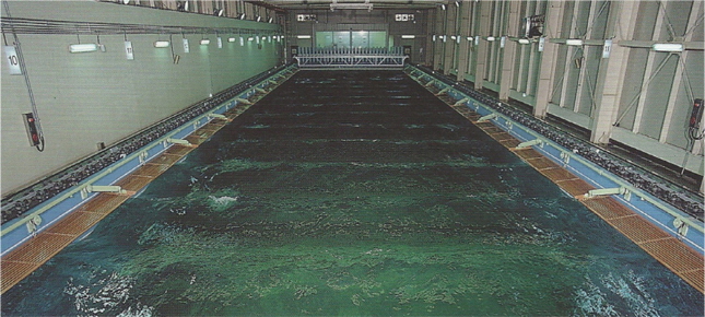
In order to verify the wave propagation scheme, the experiment is performed in wave tank. The dimension of the wave tank is 85
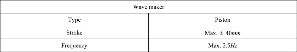
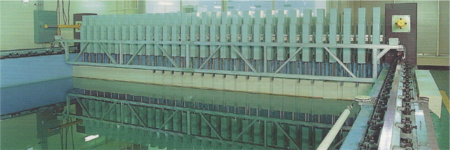
[Table 2] Specifications of wave maker.

Specifications of wave maker.
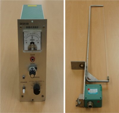
[Table 3] Specifications of wave gauge.
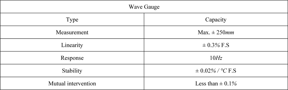
Specifications of wave gauge.
>
Wave condition and experimental set-up
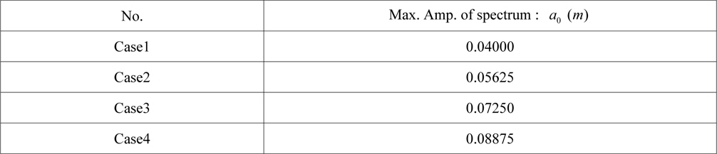
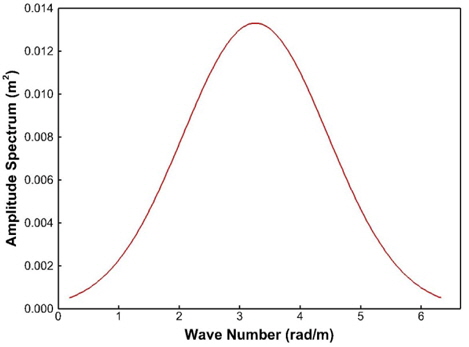
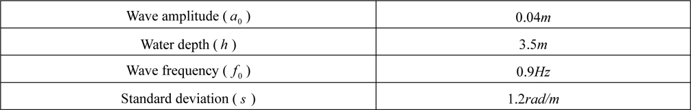
The wave spectrum with Gaussian distribution was used to generate the wave time series. As shown in Table 4, the experiment is performed with the four different maximum values of the amplitude spectrum. The water depth, the modal wave number, and the standard deviations are 3.5
[Table 4] Experimental condition of the Gaussian wave packet.

Experimental condition of the Gaussian wave packet.
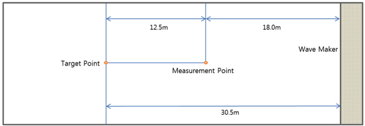
The installed position of the wave gauges is shown in Fig. 9. The measuring point and target point are located at 18.0
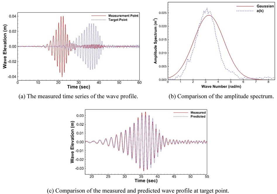
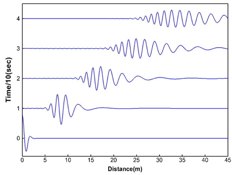
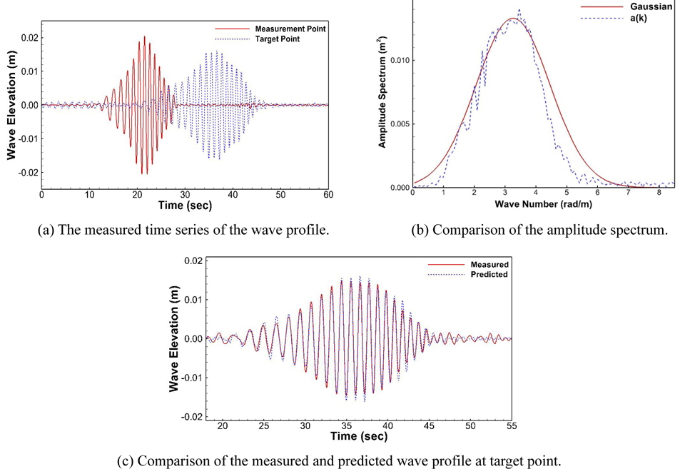
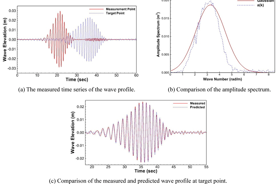
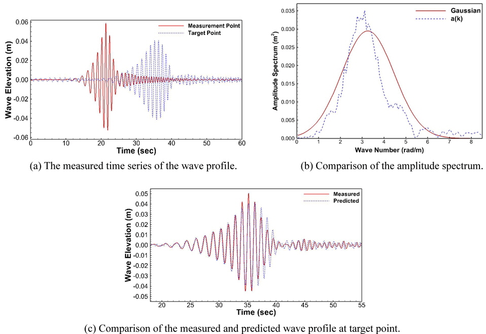
To verify the numerical method in the study, the various Gaussian wave packets are generated and measured in wave tank. The condition of the Gaussian wave packet is given in Table 4. The experimental results with our prediction model results for various Gaussian wave packets are given in Figs. 10-13. The measured wave time history is given in (a). From the measured wave profile of the front wave gauge, the amplitude spectrum can be generated. The comparison of the target amplitude spectrum with measured spectrum is shown in (b). From the spectrum we can generate wave profile at any point. To validate our model, we compared predicted wave profile with measured wave profile at target point. The comparison is shown in (c). The wave data predicted from the measured wave information agrees well with the measured result at target point. We can notice that the accuracy of the wave prediction was decreased as the wave amplitude was increased. Since the wave propagation model was based on the principle of linear superposition, we deduce that the linear characteristic influences the error of the predicted wave profile with target measurement. However, the phase of the wave profile shows good agreement for all test cases.
The wave prediction scheme based on the measured wave information is proposed. Since obtaining the wave spectrum from the measured wave data is closely related to solving an ill-conditioned matrix. Thus the solution becomes unstable. To remedy this difficulty, the ground-breaking Tikhonov regularization method is used. The Tikhonov regularization method by introducing a regularization parameter is a very efficient and reliable procedure for the stability of the final matrix and the accuracy of the numerical solution. However, there is a still another difficulty on how to choose optimized value of the regularization parameter. To overcome this difficulty, we use the L-curve method where the optimum value of the parameter is taken at the maximum-curvature point in the L-curve. The wave elevation at target point was predicted based on the wave information at measuring point to validate the proposed wave prediction scheme. It was shown that the Tikhonov regulation method using the L-curve parameter estimation give substantially reliable results. Furthermore, the proposed wave prediction scheme can be used as a valuable tool and shed some light on the research field of ocean wave problems formulated in an ill-posed problem.