The acoustic vector sensor (AVS), which measures the acoustic pressure and particle velocity simultaneously at a single point, has existed for over a century (Jia, 2009), recent advances in vector senor design have improved their utility in real engineering application (Rouquette, 2007; Lockwood and Jones, 2006; Ma et al., 2011). The AVS is advantageous for azimuth-elevation direction finding, because of the following two properties: (i) A single AVS intrinsically possesses a two-dimensional azimuth-elevation directivity; (ii) The steering vector of AVS is independent of the source’s frequency (Wu et al., 2010; Tam and Wong, 2009).

The ideal AVS and AVS array, which may be not affected by any unkown nonideality in the AVS’s amplitude response, phase response, collocation, or orthogonal orientation among its constituent velocity sensors, have been introduced and further studied by many researchers. The measurement model of the AVS array has been presented and the theoretical performance bounds on the direction finding based on AVS array has been analyzed (Nehorai and Paldi, 1994). Then, the direction finding algorithms that utilize the AVS’s unique array manifold have been developed, such as beamforming-based (Hawkes and Nehorai, 1998), MUSIC-based (Wong and Zoltowski, 2000), ESPRIT-based (Xu et al., 2007; Wang et al., 2013), and beamspace-based DOA estimation methods (Chen and Zhao, 2004). Tam and Wong (2009) and Yuan (2012) have studied how these various unknown nonidealities degrade direction finding accuracy via cramer-rao bound analysis. All above mathematical analysis and algorithms are based on the far-field measurement model, the near-field measurement model was investigated recently (Wu et al., 2010; Jacobsen and Liu, 2005). Zhou and Nehorai presented a novel approach for low frequency DOA estimation using miniature circular vector sensor array mounted on the perimeter of a cylinder (Zhou and Nehorai, 2009).

There are usually two types of acoustic vector sensors in the real engineering application, the resonant vector sensor which directly measures the particle velocity and the APGVS (Nehorai and Paldi, 1994). The APGVS is insensitive to mechanical disturbances and convenient to be installed, thus it has been used in sonarbuoy, submerged buoy and ultra-short baseline acoustic positioning systems (Chen, 2007; Wan et al., 2006). The APGVS must meet the approximation precondition ( r ≤ 0.1λ, where r denotes the radius of the APGVS and λ denotes the wavelength corresponding to the highest working frequency of the APGVS) in real engineering application. As the working frequency increases, the approximation precondition is difficult to meet, and the DOA estimation performance will degrade. In this paper, we explore the optimized methods of the DOA estimation based on single APGVS to improve the DOA estimation performance even if the radius of APGVS does not meet the approximation precondition.

This paper is organized as follows: Section 1 is the introduction, section 2 and section 3 analyze the measurement model and measurement errors of the APGVS, respectively. Section 4 analyzes several DOA estimation methods based on single APGVS and presents two modified processing methods to increase the robustness of DOA estimation based single APGVS. To evaluate the performance of the modified DOA estimation methods, numerical simulation is conducted in section 5, and on-site trial and the associated data analysis in section 6. Finally, a conclusion is drawn in section 7.

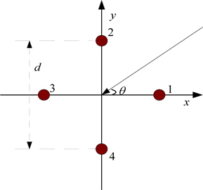
The two-dimensional APGVS is composed of four pressure sensors, whose structure can be demonstrated in Fig. 1. The acoustic pressure of the four sensors referring to the original point (the central point of the APGVS) can be denoted as

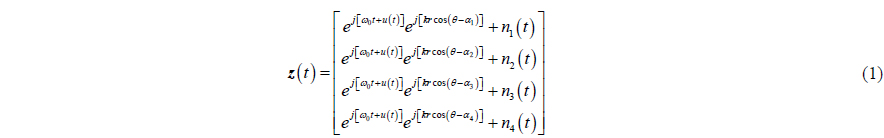
where ω₀ and u(t) are the radian frequency and the initial phase angle of the incident plane wave respectively, k denotes the wave number in water, r denotes the radius of the APGVS, and α_i( i =1,…,4) are the bearing angles of the four sensors referring to the X-axis.

Generally, the pressure of the APGVS is estimated by averaging the receiving signal of the four pressure sensors. Regardless of the system noise and ambient noise, the acoustic output pressure of the APGVS can be written as

when kr ≪ 1, the pressure in the central point of the APGVS can be further denoted as

It can be observed from (3) that when kr ≪ 1, the pressure in central point of the APGVS is equal to the average of received signals of the four pressure sensors.

The particle velocity components are usually obtained by finite difference of the pressure signal of these sensors on the same axis. Thus, the particle velocity components of the central point of the APGVS can be written as

where e^{− jπ/ 2} is added to keep the same phase between the pressure and the particle velocity components. When kr ≪ 1, the formulas (4) and (5) can be approximated as

Combining (3), (6) and (7), we can obtain a vector pattern as shown in (8) regardless of the normalization of amplitudes,

where denotes the acoustic pressure wave in the central point of the APGVS.

The APGVS did not measure acoustic pressure and particle velocity directly at a collocated point. The acoustic pressure was estimated by averaging the signals of the four pressure sensors, and the particle velocity components were estimated using pressure gradient of these sensors. Thus, the APVS has, to some degree, average and finite-difference approximation errors.

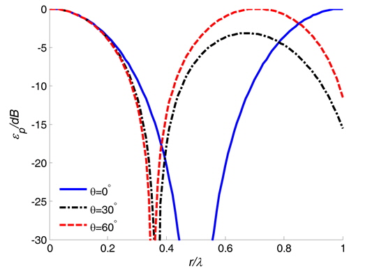
The acoustic pressure error can be evaluated by the ratio of estimated value to real value of the acoustic pressure. Frequently, we express the acoustic pressure error in dB and refer to it as “measurement error index” (Yang et al., 2013). Formulas (2) is the estimated value of the APGVS acoustic pressure, thus the measurement error index of the APGVS acoustic pressure will be

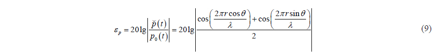
where r denotes the radius of APGVS, λ is wavelength of the acoustic signal. From (9), we can find that the acoustic pressure measurement error is determined by incident angle and the radius to wavelength ratio (Yang et al., 2013). Fig. 2 shows the curves of the acoustic pressure measurement error index with the radius to wavelength ratio for θ = 0°, 30°, and 45°, respectively. And the curves are obtained from (9). In real engineering application, the APGVS acoustic pressure measurement error index must meet the situation of |ε_p| ≤ 1dB. When θ ∈[0,2π ) and |ε_p| ≤ 1dB, the radius to wavelength ratio must meet the situation of

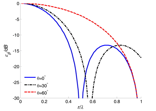
The particle velocity measurement errors index is similar to that of the acoustic pressure. The (4) and (5) are finite-difference approximation values of the two components of the APGVS’s particle velocity at central point. Considering the compensation of amplitude of particle velocity, two kinds of measurement error indexes of the particle velocity can be written as

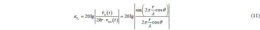
where v_0x (t) and v_0y(t) are the two components of the APGVS particle velocity at the central point. From (11) and (12), we can find that and are determined by incident angle θ and the radius to wavelength ratio r/λ . As the incident wave may come from arbitrary direction within[0,2π ) , the two kinds of particle velocity measurement errors have the same variation in θ ∈[0,2π ) . Fig. 3 shows the error index curves with the r/λ for θ = 0°, 30°, and 60°, respectively, which are obtained from (11). And whenθ ∈[0,2π ) and |ε_p| ≤ 1dB , the radius to wavelength ratio must meet the situation of

In summary, if the acoustic pressure measurement error and particle velocity errors are not bigger than 1dB, the radius of the APGVS must meet

where λ is the wavelength corresponding to the highest working frequency of the APGVS. In the real engineering application, the condition denoted by (14) is usually called the approximation precondition of the APGVS. If the APGVS radius meets the approximation precondition, the APGVS has stable working performance and its particle velocity outputs have dipole directivity, otherwise, its DOA estimation performance declines significantly. When the APGVS is working in low frequency, it is easy to achieve the approximation precondition. Instead, if the APGVS works in relatively high frequency, it is difficult to achieve the approximation precondition, which makes a higher demand of fabricating materials and structure designs of the APGVS. At another point, the approximation precondition increases the cost of the APGVS and limits its application.

Assuming the incident signal of targets and ambient noise received by the APGVS are uncorrelated, and from (8), the average acoustic intensity components can be written as

where I_x and I_y denote the average acoustic intensity of X-axis and Y-axis, respectively. Δ_x and Δ_y are the relative acoustic intensity components generated by noise. When the signal to noise ratio (SNR) is relatively high, the acoustic intensity components Δ_x and Δy can be ignored. If we divide I_y by I_x and find its arctangent, we can get

where is the azimuth estimation value of the incident wave.

The DOA estimation method aforementioned is usually referred to as “average acoustic intensity (AAI) method”. If there are multi-targets around the APGVS, the AAI method becomes ineffective, but we can utilize the difference of the incident signal spectra to distinguish them. We denote the Fourier transform of the three channels signals of the APGVS by P(ω), V_x(ω) and V_y(ω), thus, the cross spectra of acoustic pressure and particle velocity components can be written as

where the superscript * represents conjugate.

The ocean acoustic channel approximately meets the acoustic Ohm’s law, and acoustic pressure and particle velocity have the same phase. According to the properties of the Fourier transform, the azimuths of incident waves can be estimated by

where 〈⋅〉 represents moving average periodogram operator and Re{ } denotes the real value part of the entity inside{⋅} . The DOA estimation method denoted by (18) is usually referred to as “conjugate acoustic intensity (CAI) method”, which has better performance than AAI method in target detection, DOA estimation, multiple targets resolution, etc.

As the working frequency increases, it is increasingly difficult to meet the approximation precondition for the APGVS. To expand APGVS working frequency band and increase its application range, we must find new processing approaches to improve APGVS working performance (Chen, 2007).

For notational simplicity, we will omit explicit dependence on t . And if denotes the acoustic pressure autocorrelation function, and denote the cross-correlation function between the acoustic pressure and particle velocity on X-axis and Y-axis, respectively, from (2), (4) and (5), we can get

This can be put in more distinct form by simple deformation, and then we can get

Let u=kr cosθ and v=kr sinθ denote two unknowns, and solve the equations set (21), and then we can get

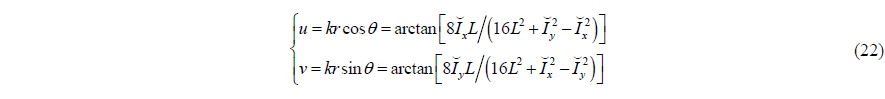
According to the relation of the trigonometric, the azimuth can be estimated by

To distinguish this approach from acoustic intensity method, it can be called “modified acoustic intensity (MAI) method”.

The minimum variance distortionless response (MVDR) beamforming of single APGVE is an extension of MVDR beamforming of array with multiple elements. We process the received signal y(t) of the APGVS with a vector operation, and make the output meet two criteria, one is the distortionless criterion and the other is minimum variance unbiased estimation criterion. According to convex optimization theory, the aforementioned process can be denoted as

where P is the output power of the APGVS, w is the weight factor, and a(θ_k) [ 1,cosθ_k, sinθ_k ]^T is the steering vector of the incident wave. is the covariance matrix estimation of the receiving data of the APGVS, which is denoted as

where y(t_n) denotes the nth snapshot of the APGVS, and N denotes the total snapshot number.

Solving equations set (24) by using a Lagrange multiplier, and the optimal weight factor w_opt can be obtained as

Substituting (26) into (24), we can obtain

where a(θ) [ 1,cosθ, sinθ ]^T is the scanning vector of the APGVS, and is its spatial spectra. We can calculate the by varying a(θ ) over θ ∈[0,2π ) and then choose its minima, thus the azimuth of incident wave is obtained. This process is called “MVDR beamforming method” of acoustic vector sensor (VMVDR).

When the radius of APGVS does not meet the approximation precondition in (14), the estimation performance of VMVDR of APGVS will degrade significantly. The main reason is the approximation error of steering vector.

From (2), (4) and (5), the accurate output of the APGVS can be written as

where is noise vector, and is accurate steering vector of the APGVS, which can be written as

The accurate steering vector is dependent on radius of the APGVS, so it has no approximation error with respect to radius variation of the APGVS. If we replace in (29) with a(θ) in (27) , the spatial spectra of the APGVS can be written as

The steering vector is accurate, thus the output spatial spectra have no approximation errors. So the estimation performance of the estimator defined in (30) won’t degrade with increase of the radius of the APGVS. In order to distinguish the process defined in (30) from VMVDR, this processing approach is referred to as “modified MVDR beamforming method” of the APGVS (MVMVDR).

In this section, we present some experiments to evaluate the estimation performance of the aforementioned four processing methods. The incident wave is the CW pulse with central frequency 7kHz and pulse width 50ms, and the sampling frequency is 50kHz. The ambient noise is assumed to be isotropic noise and all the simulation results are obtained via 200 Monte-Carlo runs.

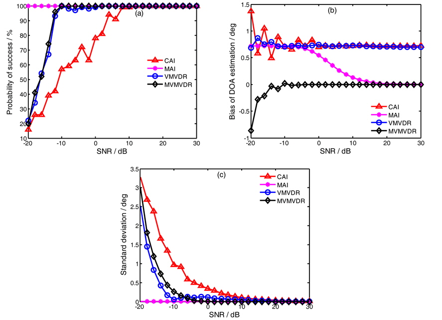
Fig. 4 shows the estimation performance of the four processing methods with the radius r = 0.02m of the APGVS. In this case, the radius to wavelength ratio is about 0.093, which is lower than 0.1, that is, the APGVS meets the approximation precondition. Subfigure (a) is the probability of success against the input SNR under the azimuth estimation limit is 1°, subfigure (b) is the bias of the DOA estimation against the input SNR and subfigure (c) is the standard deviation of DOA estimation against the input SNR. As Fig. 4 shows, we can find

(1) Under the condition of 1° error limit, the probability of success reaches 100％ when the input SNR of CAI, MAI, VMVDR and MVMVDR methods is bigger than 10dB, −20dB, 2dB, −10dB, respectively. Thus the order is CAI>VMVDR> MVMVDR>MAI for input SNR threshold of four processing methods. (2) The DOA estimation bias of CAI and VMVDR methods is about 0.73° , and there is no bias for the MAI and the MVMVDR methods when their input SNR is bigger than 20dB and −8dB, respectively. (3) The standard deviation of the MAI and the MVMVDR methods are lower than the CAI and the VMVDR methods, respectively.

From Fig. 4, we can find that the two modified processing methods have better DOA estimation performance when the radius of the APGVS meets the approximation precondition denoted in (14).

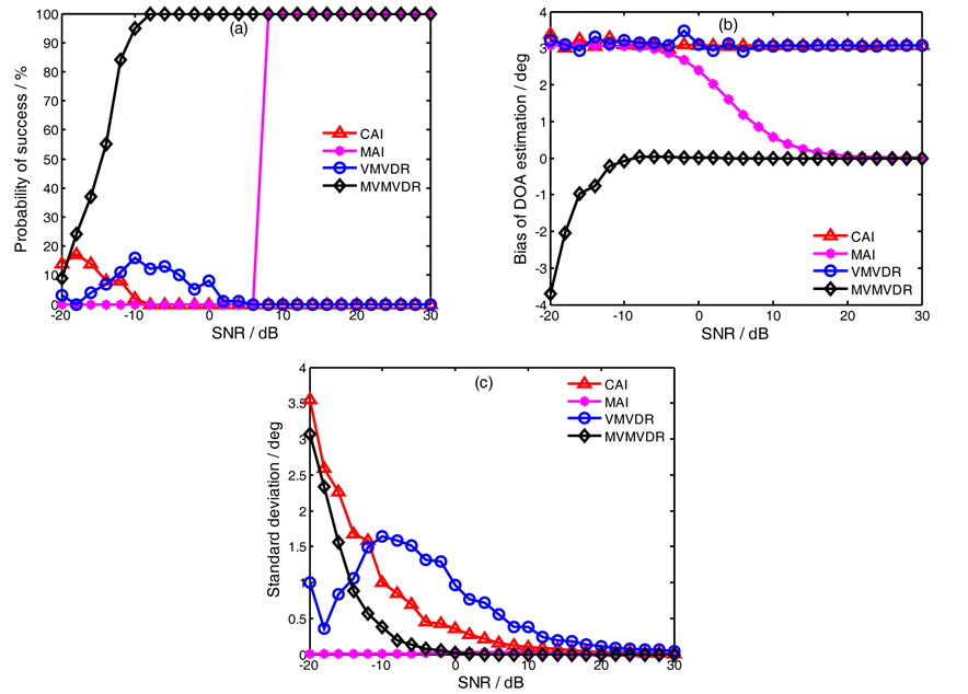
Fig. 5 shows the estimation performance of the four processing methods with the radius r = 0.04m of the APGVS. In this case, the radius to wavelength ratio is about 0.187, which is bigger than 0.1, that is, the APGVS does not meet the approapproximation precondition. The physical implication of four subfigures is the same as that in Fig. 4. As Fig. 5 shows, we can find

(1) Under the condition of 1° error limit, the probability of success of MAI and MVMVDR methods reaches 100％ when the input SNR meets SNR≥8dB and SNR≥−8dB, respectively. The CAI and VMVDR methods don’t correctly estimate the target azimuth under this condition. (2) MAI and MVMVDR methods are unbiased when the input SNR meets SNR≥−8dB and SNR≥20dB, respectively. The bias of the CAI and VMVDR methods increases to about 3.1°. (3) The standard deviation of the MVMVDR method is lower than that of the MAI method. (4) When the MAI and MVMVDR method reach unbiased estimation, their input SNR threshold is the same as in Fig. 4, respectively.

From Fig. 5, we can find that the two modified processing methods can still correctly estimate the target azimuth when the radius of APGVS does not meet approximation precondition. The MVMVDR method works better than the MAI method by about 20dB. The results indicate that the two modified processing approaches are feasible and effective compared to original approaches.

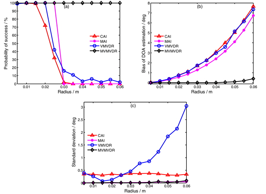
Fig. 6 studies the DOA estimation performance with different radiuses of four processing methods when the input SNR is 0 dB. Three subfigure concepts are the same as in Figs. 4 and 5. Simulation results of Fig. 6 show that the bias of DOA estimation of the four processing methods increases with the increase of the radius. The MAI method has better performance than the CAI, but its DOA estimation performance is worse than the MVMVDR method when the input SNR is small, which coincides with aforementioned results. With the highest probability of success, smallest bias and standard deviation, the MVMVDR method has the best DOA estimation performance in the four processing methods when the input SNR is relatively small.

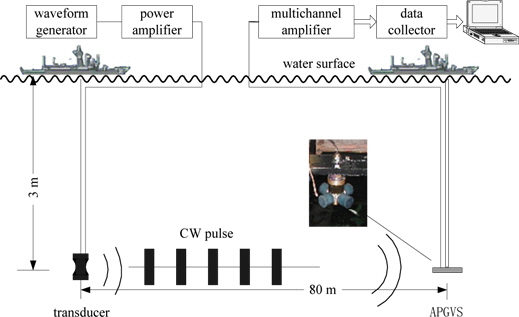
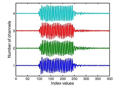
The proposed modified processing methods are applied to real underwater acoustic data collected by actual APGVS in lake water. The practical lake trial system was designed as shown in Fig. 7. The APGVS with radius 0.04m was suspended from a ship to a depth of 3m and the sound speed about 1,450m/s. The source was dragged by a moving ship at the same depth as the receiving APGVS at the distance of about 80m, and the moving ship revolved around the receiving ship. The transmitted signal was a rectangular window modulated single frequency continuous-wave (CW) pulse with a frequency of f₀= 7kHz, a duration of 2.86ms, and a repetition period of 1s. The sampling frequency of the time signal was f_s = 50kHz. Fig. 8 shows the received signal of the APGVS. The figure shows that the received signals are much stronger than the noise, that is, the signals to noise are fairly larger. In the lake trial, the radius to wavelength ratio was about 0.193, that is, the APGVS didn’t meet the approximation precondition expressed in (14).

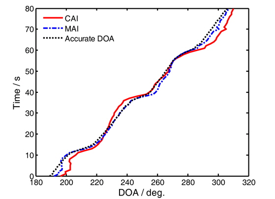
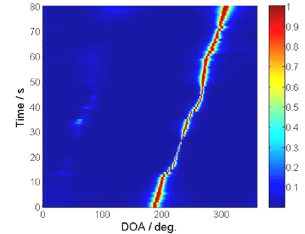
Fig. 9 shows the time-bearing display of the trial data by the CAI and the MAI methods. The ‘Accurate DOA’ in Fig. 9 is the estimation of the DOA using the data of an APGVS array, which can be regarded as the practical azimuth of the incident wave. The results are given by three curves, the solid and dashdotted curve represent the DOA estimation of the CAI and MAI methods, respectively, and the dotted curve denotes the real azimuth. From the results of 80s data in Fig. 9, we can find the curve of the MAI method is closer from the real azimuth compared with the curve of the CAI method, which indicates that the MAI method is effective for high input SNR when the radius of APGVS does not meet the approximation precondition expressed in (14).

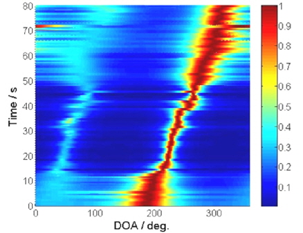
Results of the VMVDR and MVMVDR methods are shown in Fig. 10 and in Fig. 11, respectively. The two processing methods estimate the azimuth of incident wave by searching the maximum of the spatial spectra, thus the results are given in the form of time-bearing spectra surface. Comparing the results of the two processing methods in Fig. 10 and in Fig. 11, we can find that the trace of the MVMVDR method is narrower and clearer than that of the VMVDR method. The trial results are quite similar to the simulation results described in the former section, which indicates that the MVMVDR method is effective when the radius of APGVS does not meet the approximation precondition expressed in (14).

In this paper, the measurement model and the measurement errors of the APGVS are introduced, and several DOA estimation methods are analyzed. In real engineering application, the radius to wavelength ratio must meet 0≤r/λ ≤0.1 under the condition that the amplitude errors of pressure and particle velocity are smaller than 1dB. The limit of radius to wavelength ratio is usually called “approximation precondition”. Two modified processing methods (the MAI and MVMVDR methods) are presented to improve the DOA estimation performance of the APGVS when it does not meet the approximation precondition. Finally, the simulation and lake trial are conducted to evaluate the performance of the two modified processing methods. From the results, we can conclude: (i) the two modified processing methods have better DOA estimation performance than original processing methods when the radius to wavelength ratio of the APGVS isn’t bigger than 0.1. (ii) The two modified processing methods can successfully estimate DOA of incident wave when the radius to wavelength ratio is bigger than 0.1. (iii) The two modified processing methods are unbiased when the signal to noise ratio is relatively high, and the MVMVDR method works better than the MAI method by about 20dB.