In computer vision, a feature can be defined as an interesting part or point of an image, as in [1]. A feature contains some information which apart from its neighborhood. It means that the feature is considered distinctiveness within a certain range. These features could be shape, texture, color, edge, corner and blob etc. Features have high informative contents and appear over and over again in different images. They may be described by the shape, edge or color of objects, or the correlations between two or more images or objects. Until now, many image processing algorithms are based on image feature such as photo stitching, self-localization of robot, objects recognition, object tracking and 3D reconstruction.

In [1], image feature detection refers to methods to compute abstraction of image. Tuytelaars and Mikolajczyk [2] addressed an overview of invariant interest point detectors, how they evolved over time, how they work, and what their respective strengths and weaknesses are. The three robust feature detection methods scale invariant feature transform (SIFT), principal component analysisSIFT and speeded up robust features (SURF) were summarized in [3]. In [4], blob feature detection is defined as one of feature detection. The blob detection is a mathematical method which detects regions or points in a digital image. The regions or points have noticeable difference with their neighborhood. Additionally, a blob is a region or point in which some properties are invariant within a prescribed range of values. Kim and Seo [5] introduced genetic programming based corner detectors for an image processing. In [6-8], some applications for image processing were presented.

In this paper, we present that how some existed corner and blob feature detection algorithms work and how long they execute for an analysis of some different algorithms. And we also discover the application context for each algorithm. The related works are presented in Section 2. In Section 3, the overview of the corner and blob feature detection algorithms are discussed. Some experiments and simulation results are shown in Section 4. We describe some discussions and future works in Section 5. We here see that Harris corner detection can detect a large number of interest points, but they contain less information for interest point region. Difference of Gaussian (DoG) and determinant of the Hessian (DoH) have similar results in interest point detection, but DoH has faster than that of DoG.

In 1988, Harris and Stephens [9] proposed a method to detect a corner of an image, which is later called Harris Corner Detector. The method is based on the eigenvalues of the second-moment matrix. The Harris Corner can detect robust corner of an image. However, the algorithm only detects the location of corner, and avoids the interest points which not belong to the corner.

In 1997, a new algorithm called features from accelerated segment test (FAST) was proposed for corner detection. The most contribution of FAST is its computational efficiency. Comparing with other well-known feature detection algorithms such as Harris Detector, smallest univalue segment assimilating nucleus and DoG, it is so faster. So, FAST has been applied in many real time applications such as cleaning robot.

Laplacian of the Gaussian (LoG) is one of the first and also most common blob detectors. The blob feature can be detected from different scale. In comparison with corner algorithms, the scale-space theory is leaded into for detecting interest point of image and a blob contains more information than a corner feature. It means that the point can be described by its neighborhood around it. The feature detection is performed to blob detection from corner detection. In 1999, Lowe used DoG to replace LoG for detecting the interest point with rapid calculation.

Because Hessian matrix has a good performance in accuracy, DoH was also used for detection of the blob feature. In 2006, Bay and Tuytelaars used the scale-normalized DoH from Haar wavelets to detect the interest point. From their experiment results, DoH has similar effect in the interest point detection with DoG, but it is three times faster than that of DoG.

In order to detect image features which are invariant through image affine transformation, Mikolajczyk and Schmid [10] proposed Harris affine detector in. Harris affine detector identifies initial blob using Harris-Laplace detector and then normalizes the blob using affine shape adaption. And the blob is estimated iteratively. The algorithm can identify similar regions between images. However, the algorithm expends a great of time.

For the comparison of several algorithms, we describe the implementation of the detection methodology by step

Let the image be given by I,

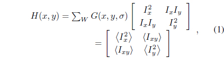
where H stands for a Harris matrix, Wis weighted window, I_x and I_y is the partial derivatives of I, and G(x, y, σ) is Gaussian matrix and expressed in Eq. (5).

For each pixel, Harris and Stephens used Eq. (2) to compute corner response for the computational efficiency,

where k is a tunable sensitivity parameter. If the M_c of the point is greater than the given threshold, the point is considered to be a corner.

Kanade and Tomasi [11] computed directly the M_c by Eq. (3):

where λ₁ and λ₂ are the eigenvalues of H.

A large number of experiments have approved that the method is better results because the corner is more stable for tracking.

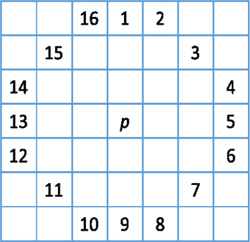
The FAST uses a circle of 16 pixels to determine whether the center of circle is a corner, like Figure 1.

1) Assume that the intensity of the center of the circle is Ip. Set a threshold intensity value T.2) For fast computing, Ip is first compared to the intensity of pixels I1, I5, I9, and I13. If at least three pixels of these four pixels are all brighter than Ip + T or darker than Ip − T, the corner will exist. If not, it will be quit.3) If a set of N contiguous pixels out of the 16 needs to be either above or below Ip by the value T, then Ip is a corner.

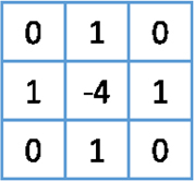
The Laplacian is a 2D isotropic measure of the second order derivative of an image. The Laplacian L(x, y) of the original image I is given as follows.

Because the original image is represented as a set of discrete pixels, the Laplacian can be approximated by using a discrete convolution kernel as shown in Figure 2.

Because the Laplacian filter is very sensitive to a noise, it is common to smooth image using a Gaussian kernel of Eq. (5) before applying the Laplacian filter.

So, the two-step process is called LoG operation. The overall process for LoG is as follows:

In order to detect the blob features which are invariant in different environment, a multi-scale σ is used to filter the original image. A scale-normalized approach is necessary to obtain a multi-scale blob detector with automatic scale selection as the following Eq. (7).

The points are considered as the interest points (blob feature) which are local maxima or minima of

Similar to LoG, the image I is first smoothed by convolution with Gaussian kernel of a certain widthσ. Then a different Gaussian kernel σ + ∆σ is used to smooth the original image again. The difference of these two Gaussian smoothed images is called DoG, as the following Eq. (9).

In fact, DoG is a band-pass filter, which can remove high frequency components representing noise and some low frequency components representing the homogeneous areas.

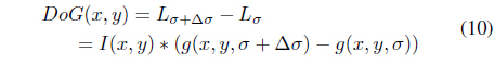
The DoG is one of applicants for edge detection and blob detection in image processing algorithm. The best known application is a keypoint detection proposed by Lowe [12] in 2004.

For fast computing in [12], DoG is defined as an operator or a convolution kernel like the following Eq. (10).

The Hessian matrix is a square matrix of the second partial derivatives of the function and it could be described by the local curvature of an image as mentioned in [13].

Similar to LoG, DoH considers scale-space to detect the interest points.

The interest points are selected using the following function to find maxima in scale-space.

DoH was used in SURF [10], the detection effect of the interest points is similar with SIFT. However, the detection time is three times faster than that of the SIFT through integral image used.

According to affine-invariant theory and multi-scale Harris corner points detection theory, Harris affine detector uses following iterative methods to detect interest points.

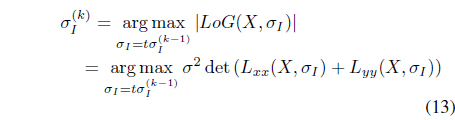
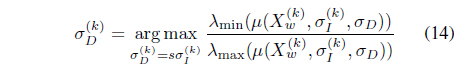
1) Initialize the search space through Harris-Laplace detector. U(0) = Identity Matrix E2) Normalize ellipsoid region to circle region using the shape adaptation matrix which generated in pervious iteration U(k−1), center in = U(k−1)−1X(k−1) 3) Select the integration scale, . The is determined as the scale that maximizes the LoG.4) Select the derivation scale, . The derivation scale is taken to be related to the integration scale through a constant factor: , where s ∈ [0.5, ··· , 0.75], and

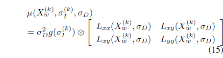
where µis the second moment matrix, and λmin and λmax are the Maximum and Minimum eigenvalues of the matrix µ, respectively. µ is also defined as

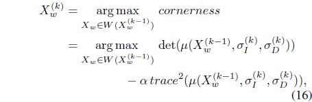
5) Spatial localization: select the point that computes the Harris corner measure (cornerness) within an 8-point neighborhood around . Find the maximum in the neighborhood, is as follows:

where the window W() is the set of 8-nearest neighborhood of the pervious point.

Compute the location of interest point X(k)

6) Update the shape adaptation transformation matrix U.

where

7) Compute the stopping criterion. Suficiently close implies the following stopping condition.Mikolajczyk and Schmid had good result with εc = 0.05.

Meanwhile, a detection algorithm called Harris affine region detector are proposed. The Harris affine detector relies on the combination of corner points detected thorough Harris corner detection, Gaussian scale space, and affine shape adaptation algorithm. And like the Harris affine algorithm, the Hessian affine replaces Harris matrix using Hessian matrix for detecting affine interest points.

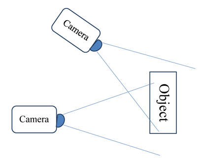
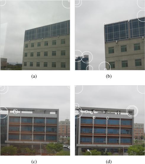
In this Section, some simulation results of corner and blob detection algorithm will be presented. For comparison, two sets of images are selected for simulation. The images were captured in different view perspectives as shown in Figure 3.

According to the method in Section 3, we use four images for the simulation. The simulation results are shown as followings.

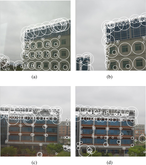
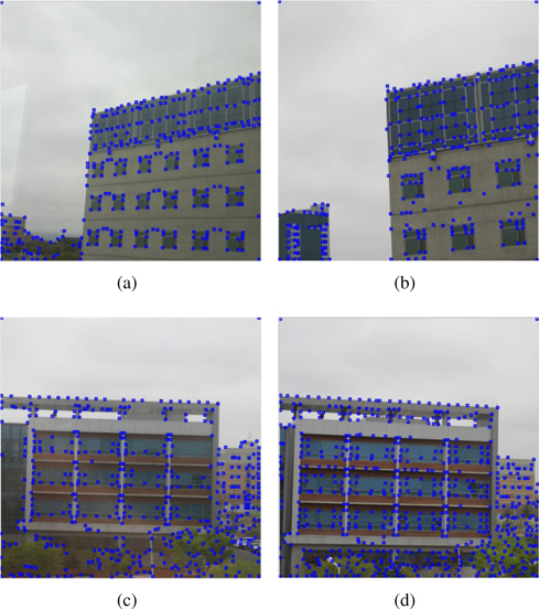
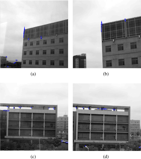
From two set of images in Figure 4, a large number of corners are detected. In the same position of two images, the same corners were detected.

Scale-space has been led to detect interest points. The interest point not only contains the coordinate, but also the scale which descripts an effect of interest point to its neighbor.

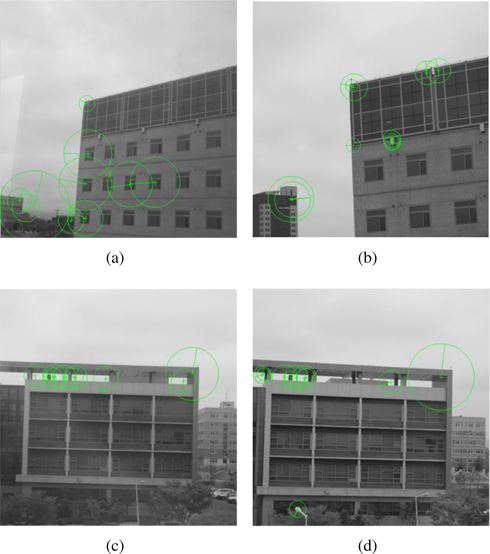
From Figure 5, the detected interest points are less than that of Harris corner detection algorithm and its computation speed is also slower.

Because of similar results between LoG and DoG, the scalespace has been used for Harr corner detection, which is called Harris Laplace detection.

From Figure 6, the results have a smller number of interest points. The computing time is similar to that of LoG.

In DoH, integral image has been led to fast detection of interest points. The computing time is also three times faster than that of LoG.

The figure 7 shows interest points detected by DoH algorithm. The great advantage of DoH is computing time. If scale-space is not particularly large, DoH can be used for real-time interest points detection.

For the affine transformation and denser descript object, affine shape adaptation is used. The feature of images is not descripted by a circle such as those of LoG and DoH, but an ellipse.

From Figure 8, each interest point contains an ellipse region. We could see that the ellipses have similar pixels and similar orientations by the comparison of two sets of images. This provides great convenience for more accurate matching in two images. However, the iterative time for learning is equally vast.

In this paper, a comparative analysis for some corner and blob detection algorithms has been done. Harris corner detection can detect a large number of interest points and has good performance in interest point’s robust and computing time. These points can reflect texture of objects. However, these points contain less information for interest point region. Through scale-space has led to detect interest points of image, the interest points have been replaced by blobs. The blob is easier to reflect the feature of interest point region in different environment change such as illumination, rotation and scale of images. For simulation results in DoG and DoH, both have similar result in interest point detection, but DoH has faster than that of DoG. Harris affine region detection algorithm added affine shape adaptation for region normalization. The blob detection satisfies image affine transformation. However, the computing time and complexity are much increased by the iteration.

No potential conflict of interest relevant to this article was reported.