Axially distributed image sensing (ADS) systems are capable of acquiring 3D information for 3D objects or partially occluded 3D objects [1-6]. The ADS scheme can provide simple recording architecture by translating a single camera along its optical axis. The recorded high-resolution elemental images generate the clear 3D slice images for the partially occluded 3D objects compared with the conventional integral imaging method [6-16]. The capacity of this method to collect 3D information is related to the object location from the optical axis. The 3D information cannot be collected when the coordinates of the object are close to the optical axis (i.e., on axis).
Recently, the resolution analysis methods to evaluate the performance of a 3D integral imaging system under the equally-constrained resources have been reported [17-19]. The lateral and longitudinal resolutions of the given 3D integral imaging systems by considering several system parameters such as the number of sensors, pixel size, imaging optics, relative sensor configuration, and so on.
In this paper, we present a framework for performance evaluation of ADS systems under the equally-constrained resources such as a fixed number of pixels, a fixed moving distance, a fixed pixel size and so on. For the given ADS framework, we analyze depth and lateral resolutions based on the two point sources resolution criterion [17] where two point sources and a spatial ray projection model are used. The Monte Carlo simulations are carried out for this analysis and the simulation results are presented.
II. RESOLUTION ANALYSIS FOR ADS SYSTEM
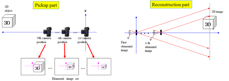
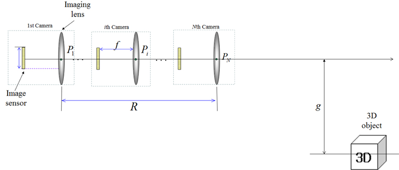
The typical ADS system is shown in Fig. 1 where a single camera is moved along the optical axis. The different elemental images are captured along the optical axis if 3D objects are located at a certain distance. Each elemental image has the different scales for 3D objects. On the other hand, the digital reconstruction process of 3D objects is the inverse process of pickup. 3D images can be obtained using computational reconstruction based on an inverse mapping procedure through a virtual pinhole model [3]. In fact, ADS pickup structure is highly related to the resolution of 3D reconstructed images. In this paper, we want to evaluate the performances of ADS according to the pickup structure.
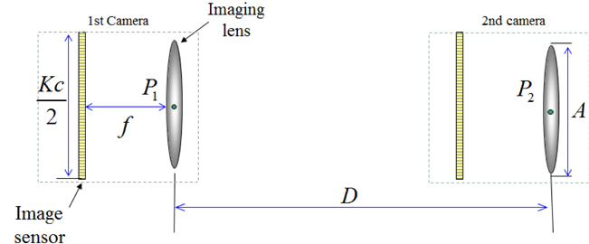
Figure 2 illustrates the general framework of ADS system with
In the ADS framework as shown in Fig. 2, we can vary the number of cameras
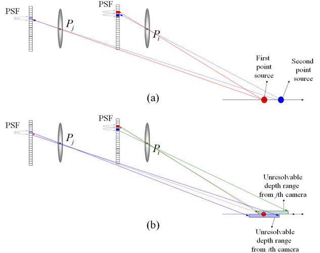
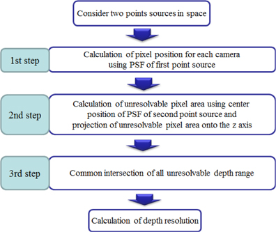
In order to analyze the resolution performance for the ADS framework of Fig. 2, we utilize the resolution analysis method based on two point sources resolution criteria [17], which is defined as the ability to distinguish two closely spaced point sources. The principle of the resolution analysis used can be explained through three steps as shown in Fig. 4. We consider only one-dimensional notation for simplicity. We assume that there are two close point sources in space.
The first step is to find the mapping pixel index for the first point source located at (
where
where is the rounding operator.
The second step is to calculate the unresolvable pixel area for the mapping pixels calculated in the first step. The unresolvable pixel area means that two point sources can be separated or not. That is, when the position of the second point source is closely located to the first point source, we can resolve two point sources if the second point source is registered by at least one sensor so that it is in a pixel that is adjacent to the pixel that registered the first PSF. But, if the second PSF falls on the same pixel that recorded the PSF of the first point source, we cannot resolve them. In this analysis, the unresolved area is considered to analyze the resolution. Thus, the possible mapping pixel range of the second point source is given by
We can calculate the unresolvable pixel area of the second point source for the mapping pixel using ray back-projection into the plane of two point sources. It is presented by
In the third step of resolution analysis, we will find the common area for the unresolvable pixel areas calculated from all cameras. The depth resolution can be considered as the common intersection of all unresolvable pixel ranges. Thus, the depth resolution becomes
The computational experiments are carried out for the depth resolution of various ADS frameworks. The two point source resolution analysis method was used to calculate their depth resolutions as described in the previous section.
Based on two point sources resolution analysis, the Monte Carlo simulations are performed to statistically compute the depth resolution for various ADS frameworks. Two point sources are placed longitudinally to determine the depth resolution. The first point source is located randomly in space and the second point source is moved in the longitudinal direction. The experimental conditions for the Monte Carlo simulation are shown in Table 1.
[TABLE 1.] Experimental constraints for Monte Carlo simulation.
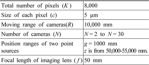
Experimental constraints for Monte Carlo simulation.
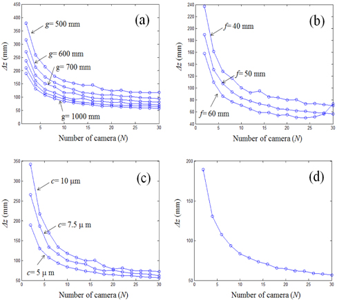
The Monte Carlo simulations were repeated for 2,000 trials where the locations of two point sources were selected randomly. After that, the depth resolutions were calculated as the sample mean. The simulation results of depth resolution for ADS frameworks are obtained while changing several system parameters. First, the simulation results of depth resolution according to the number of cameras are shown in Fig. 6(a). Here, several distances (
In conclusion, a resolution analysis of various ADS frameworks under fixed-constrained resources has been presented. The system performance in terms of depth resolution as a function of system parameters such as the number of cameras, the number of pixels, pixel size, and focal length were evaluated. It has been shown that the depth resolution in an ADS system can be improved with the large number of cameras and the large distance between optical axis and point source plane. We expect that the proposed method can be useful to design a practical ADS system.