A micro zoom system without moving elements by use of two liquid lenses is designed and optimized in this paper. The zoom equations of the system composed of two liquid lenses are deduced. The structure parameters including radius and thickness of a conical double-liquid electrowetting based lens are analyzed and calculated. Because the liquid thickness varies non-linearly with the radius of the interface, it’s very difficult to optimize a real liquid lens using commercial optical design software directly. Through the Application Programming Interface (API) of the optical design software CODE V, a zoom system with two real electrowetting based liquid lenses is modeled and optimized. A two-liquid-lens zoom system without moving elements, with a zoom factor of 1.8 and a compact structure of 10 mm is designed for illustration. This can be useful for the camera design of mobile phones, tablets and so on. And this paper presents a convenient way of designing and optimizing a zoom system including liquid lenses by commercial optical design software.
Miniature zoom systems are widely used for many advanced optical systems today. The conventional zoom system always has more than two elements with nonlinear movement to implement focus variation and imaging shift compensation at the same time. This will lead to large volume and complicated structure of the system. The liquid lens is a novel type of optical device. With the character of active zooming, the liquid lens can make a zoom optical system more miniature, and has very wide potential applications in mobile phones, micro projectors and so on.
There are three main types of tunable-focus liquid lenses: liquid crystal lens [1-2], electrowetting effect based liquid lens [3-5] and liquid-filled membrane lens [6-8]. The electrowetting effect based liquid lens was first reported by the researchers of Philips Optical in 2003 in [3]. The focal length can be adjusted under different external voltages by changing the curvature of the interface between two kinds of immiscible liquids. This kind of liquid lens has short response time and wide focus tunable range. Now Varioptic can provide a series of commercial products of this kind of liquid lens.
By use of the liquid lens, zoom optical systems can be designed without moving elements. This will avoid many disadvantages of conventional zoom systems, which may be complicated, fragile and expensive. Some researchers published results and analysis of zoom optical systems with variable power liquid lenses. Kupier [4] pointed out that more than two liquid lenses are required to implement a zoom system. Zhang [9] analyzed the principle of the two liquid lenses zoom system by Gaussian optics. The paraxial and third order aberration and first order chromatic aberration analysis of zoom systems based on liquid lenses were studied in [10]. Sun, Park and Fang [11-13] gave examples of the zoom system design with a liquid lens and one group of moving lenses. But the zoom system with no moving elements has not been discussed. And much research has been reported to try to design zoom systems with liquid lenses in [14-16]. However there is still not a comprehensive method to set up a zoom system with liquid lenses, nor a convenient way to optimize the system by using commercial optical design software.
In this paper, we focus on the similarity of the zoom system with liquid lenses. The zoom equations of the system composed of two liquid lenses are deduced. The characters of the structure parameters of the conical doubleliquid electrowetting based lens are analyzed and calculated by Matlab software during the focal length change. Through the Application Programming Interface (API) of the commercial optical design software CODE V, a real liquid lens model is set up and a zoom system with liquid lenses is optimized successfully. This will make the design of the zoom system with liquid lenses much more convenient. Then a two-liquid-lenses zoom system without moving elements is designed for illustration, which has a zoom factor of 1.8 and a compact structure of 10 mm. This may be useful for a mobile phone camera, a tablet camera and so on.
II. ZOOM EQUATION OF TWO-LIQUID-LENS VARIABLE FOCUS SYSTEM
The variable focus system must satisfy two basic conditions, which are: adjustable focal length, and fixed image plane. To satisfy the two conditions at the same time, there need to be more than two pieces of liquid lens. One is for focal length tuning and the other is for imaging shift compensation.
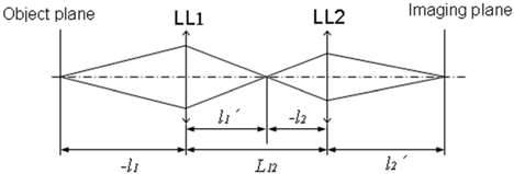
A two-liquid-lens zoom system is shown in figure 1. In the system, the liquid lens 1 (LL1) is for changing the focal length; while the liquid lens 2 (LL2) is for compensating the imaging shift.
In Fig. 1, the system is composed of only two pieces of liquid lens.
Since the conjugate distance between the object plane and the imaging plane of the system is fixed, the
According to the geometric relationship, and
Since
Presuming the focal length of LL2 (presented by ) is fixed, the image distance will be altered with the shifting of
On the other hand, presuming
Since the image distance of LL2 (presented by
According to the equations (3), (4), (5), the relationship between
According to the Gaussian Optics theory, we can get equation (7):
According to the equations (1), (2), (6), and (7), the differential function of and is gotten:
Solving the equation (8), we get the general solution:
where
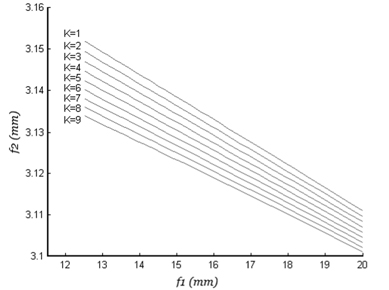
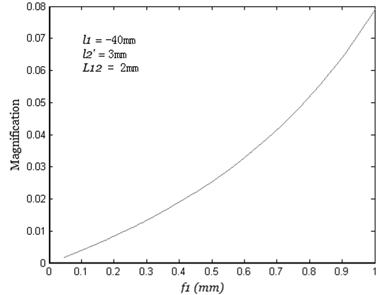
The relationship between the magnification of the system and is given by the formula (10) and is shown in Fig. 3.
According to the magnification needed and the variable range of the liquid lens, the initial system can be set up by solving the zoom equation.
III. METHODOLOGY OF OPTICAL DESIGN FOR A VARIABLE FOCUS SYSTEM WITHOUT MOVING ELEMENTS
3.1. Structure Parameters of the Conical Double-liquid Electrowetting Based Lens
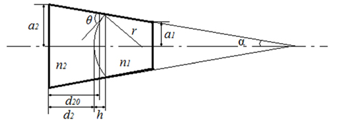
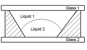
Several years ago researchers of Philips Optical announced a kind of electrowetting effect based liquid lens as a varifocal component. This type of liquid lens is composed of a cylindrical cavity and two kinds of immiscible liquid. One is conducting and the other is insulating. The refractive index of the two kinds of liquid is different. The interface of the two immiscible liquids would be perfectly spherical if the density of the two kinds of liquid were the same [15]. The contact angle of these two kinds of liquid and the cavity insulating wall (θ in Fig. 4) can be influenced by an external electric field for the electrowetting effect. Then the curvature between the two immiscible liquids can be changed and the focal length can be adjusted.
Figure 4 shows a simplified schematic of the electrowetting based liquid lens with conical structure (This structure is applied in the liquid lens of Varioptic). When the curvature between the two immiscible liquids is changed, the position of the summit of the spherical interface will be altered at the same time.
Considering the lens shown in Fig. 4,
Presuming the volume of liquid 2 is
Where
Since the volume of each liquid is constant,
According to the geometrical relationship, we can also get the following formula:
Then
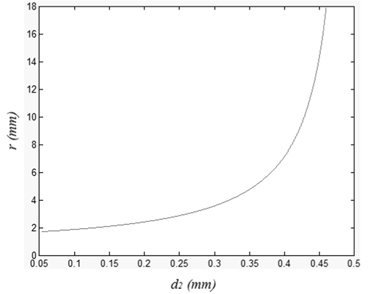
The liquid thickness and the radius of the interface are calculated according to formulae (12) and (14) by use of Matlab software. Figure 5 gives the details of the calculation, where
Like a parallel plate, the thickness change of each liquid will cause spherical aberration and spherochromatism. Presuming that the initial thickness is the thickness when the interface is plane, the maximum spherical aberration caused by the thickness change is as follow:
As an illumination, for one type of Varioptic liquid lens, the maximum change of the thickness of each liquid is about 0.2 mm. According to equation (15), the maximum spherical aberration caused by thickness change of one liquid lens is approximately 0.00024
3.2. System Set Up and Optimized
We use a commercial software (CODE V) to do the system design. The optimization is based on a damped least square (DLS) algorithm. Since the structure parameters (eg. thickness and interface radius) of the liquid lens are quite non-linear, the optimization process will be very complicated. Thanks for CODE V API (Application Programming Interface) we can realize the optimization process by using Microsoft Visual Basic (VB) to control the structure parameters of the liquid lens.
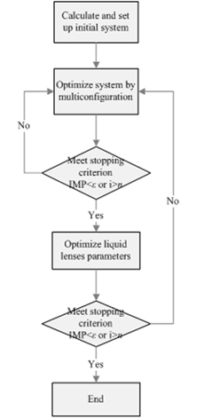
The CODE V API is an application programming interface designed to allow access from other programs to CODE V commands, which uses the Microsoft Windows standard Component Object Model (COM) interface. This enables us to execute CODE V commands using applications such as Microsoft Visual Basic (VB), Matlab, C++ and so on. By use of this, the liquid lens can be modeled and optimized. Figure 6 shows the flow chart of the optimization process.
First, we calculate the initial structure and then optimize it by multi-configuration in CODE V. In this step, the thickness and interface radius of liquid lens are not strictly constrained. Second, we optimize the two liquid lenses for every zoom. The parameters of the two liquid lenses are strictly constrained and calculated by VB. And the parameters of the liquid lens are discretized for use during this optimization process. In this step, the optimization process may take a lot of time because of the need for multiple data exchanges between VB and CODE V. To enhance the feasibility, the parameters of the system are all frozen except the thickness and interface radius of the two liquid lenses. A stopping criterion which consists of max loops number and improvement (IMP) of error function (EF) is set up before the optimization,. The optimization process is based on damped least square (DLS) algorithm. The error function (EF) is defined as follows:
where
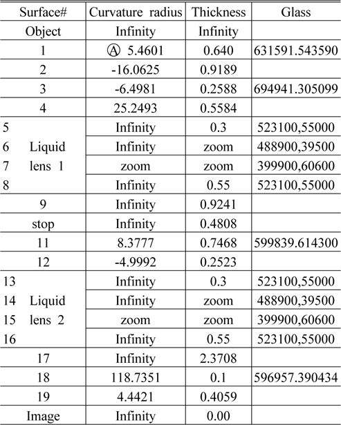
A two liquid lens zoom system is designed in this section. The long focal length of the system is
The liquid lens parameters are based on Varioptic liquid lens ARCTIC 416. The structure of the lens is shown in Figure 7 (the material of glass1 is same as that of glass2). Lens details can be seen from www.varioptic.com. The lens data of the liquid lens thickness and radius are discretized for use.
The specification of the system is shown in Table 1.
[TABLE 1.] Specification of the two liquid lens zoom system
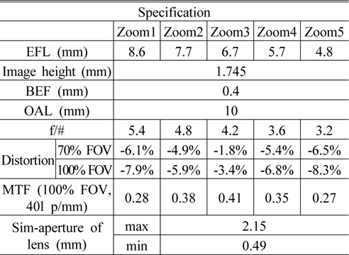
Specification of the two liquid lens zoom system
The initial system structure is calculated according to Section 2. To realize the system, three groups of classical lenses are adopted to eliminate the aberrations. The first group of solid lenses is in front of the system, which is used to eliminate the incident angle of the chief rays. The first surface of the first lens is set aspherical to balance the off-axis aberration. The second solid lens is put behind the aperture to bear part of the optical power. The third group of solid lenses with slight negative power is behind the second liquid lens, which is set to eliminate the aberration when the liquid lens has a strong positive.
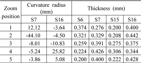
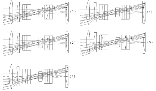
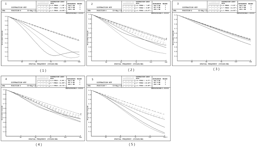
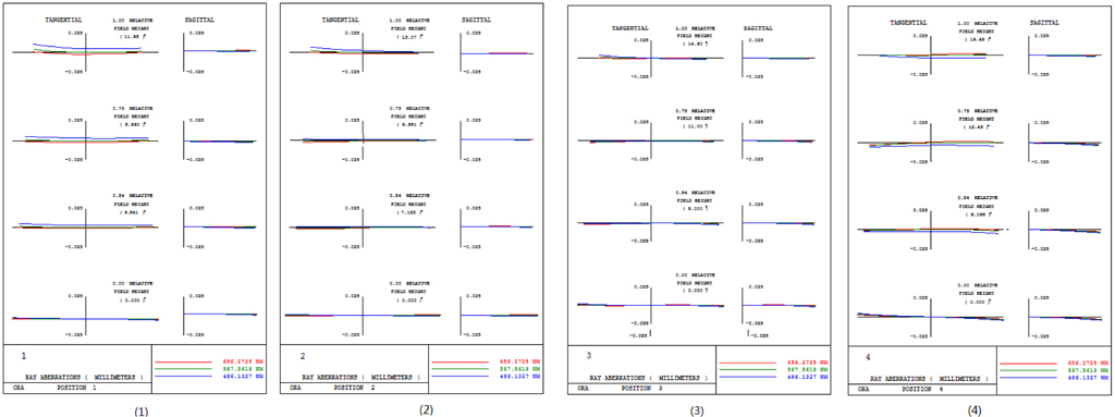
The general parameters of the system are shown in Table 2. The zoom parameters of the system are shown in Table 3. The layout of the system at different zoom positions is shown in Fig. 8. The Fig. 9, 10 show the imaging performance of the system.
[TABLE 2.] General parameters of the system

General parameters of the system
[TABLE 3.] Zoom parameters of the system

Zoom parameters of the system
A liquid lens can help a zoom system become more miniature than before due to its character of active zooming. This has a very wide potential application in many areas. In this paper, we try to give a method for designing and optimizing a zoom system including liquid lenses. First the zoom equation of the system composed of two liquid lenses is deduced. Then the structure parameters of the conical double-liquid electrowetting based lens are analyzed and calculated by Matlab software. It is shown that the liquid thickness varies quite nonlinearly with the interface radius in a liquid lens. Through the API of the commercial optical design software CODE V, the zoom system with liquid lenses is modeled and optimized successfully. The optimization process flow chart is given. The structure parameters of the liquid lens is strictly constrained and calculated by VB during the optimization. A zoom system is designed for illustration, in which two pieces of liquid lens and four pieces of traditional lens are used and a zoom factor of 1.8 is implemented. The overall length of the system is 10 mm. This has potential application in mobile phone cameras or tablet cameras.