As the essential techniques for the CD (Critical Dimension) measurement of the LCD pattern, there are various modules such as an optics design, auto-focus
In accordance with a trend of TFT-LCD panel’s enlargement, the requirement of CD measurement accuracy for each process of TFT-LCD manufacture is getting stricter. In order to improve the contrast of edges for the CD measurement, reflected light type optics is devised and applied, that has the same effect as with transmission light. Finally, a new sub-pixel algorithm is developed which complements the previously proposed sub-pixel algorithm for edge detection. We applied this system to the CD measurement process, and analyzed the results.
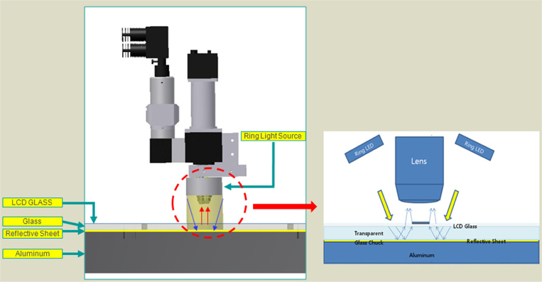
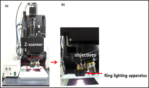
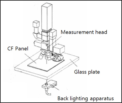
Figure 1 shows the devised system. This system consists of the ring type of reflected light which has the same effect as with the transmission light, lens, glass surface plate, aluminum surface plate, reflected sheet between glass and aluminum surface plates and a camera as an imager.
III. RING TYPE OF THE REFLECTED LIGHT OPTICS
The difference of intensity value around the edge between the object and the background is a very important factor in the CD measurement. It affects the CD measurement as well as the calculation of the focus position. In the CD measurements system, the light apparatus is divided into two types. The first is reflected light apparatus and the other is transmission light apparatus. Usually reflected light optics are useful to inspect the overall appearance of the inside of objects, but transmission light is more useful to improve the contrast of edge for CD measurement. However there are disadvantages of applying the in-line CD measurement system using transmission light. For example, the transmission light apparatus and optics must be in the opposite direction based on the glass plate. Also the system using transmission light must use fragile materials such as glass for the sample support.
In addition, the transmission light system has more complicated structure compared to the reflected light system, as the optics and transmission light under the glass plate must be moved in synchronization. So in this study, we devised a system which is a reflected light type, but has the same effect as with the transmission light. The designed optical system is shown in Fig. 3.
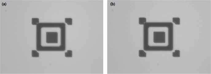
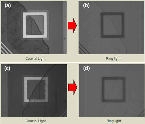
Figures 4(a) and 4(b) show the captured overlay pattern images by transmission light optics and the designed ring light optics respectively. No significant difference was found.
In addition, the unnecessary marks that can potentially cause errors in CD measurement of normal coaxial reflected light optics were remarkably reduced in the devised ring light type optics. (Fig. 5)
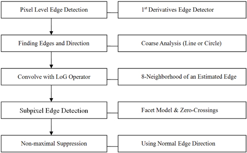
Edge detection is the preprocessing level of images for CD measurement. It senses the change of light and shade, then distinguishes the object from the background. There are Sobel, Laplacian, LoG(Laplacian of Gaussian) and Canny edge detectors that have the accuracy of the pixel level. Based on the results extracted by edge detection of pixel level, it is possible to detect the edge at the subpixel level, such as by interpolation and by the method that models the intensity of images by a parametric model[9-10]. In this study, we first detected the edge by the LoG operator of the pixel level and then conducted the subpixel level detection using facet modeling.
The edge of an object is a very important clue as it can connect an image with its interpretation. Edge detection is conducted usually by convolution that uses the surrounding pixels of a narrow area, as in work by Kirsch and Sobel. These operators are easy to use and calculate quickly, but are very sensitive to noise and highly dependent on the magnitude of objects. To compensate for these disadvantages, the operator of edge detection by zero-crossing of second order derivative was applied. This is based on the fact that the result of the first order derivative has the maximum value in the edge of the image, and the result of the second order derivative is zero on the same spot. To get the second order derivative figure of the image, we employed a smoothing filtering. This process reduces noise. The smoothing filter here that we used is 2D Gaussian G (x, y).
In the above equation, σ is the standard deviation of the probability distribution. The standard deviation
Due to the linearity of the LoG, the convolution and differential operation can be interchangeable. The form is as follows.
The above equation ∇2
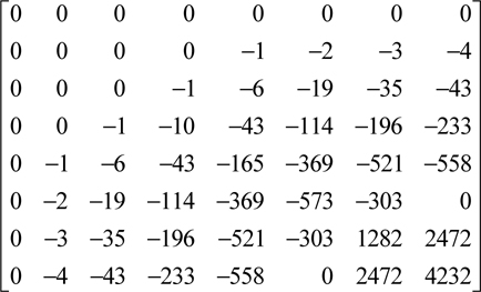
K is a scale factor and makes the sum of all LoG components zero. When
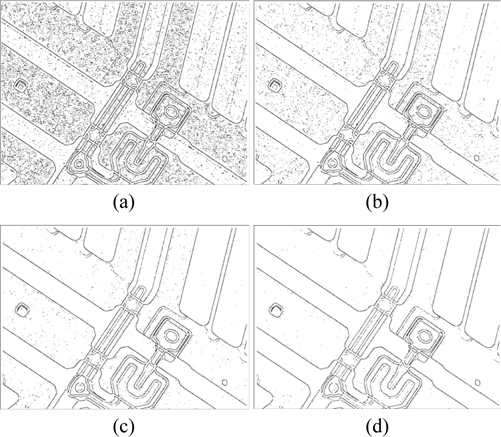
This is the upper left part of the matrix because it has a symmetry structure up and down and right and left. We conducted the edge detection for the sample image of TFT-LCD, using the LoG from the above. While we detected the edge, we changed the threshold by 90%, 70%, 50% and 20% of the edge’s maximum size. The result shows that the higher we make the threshold, the smaller noise edges appear.
In general, there are two types of subpixel edge detection methods, the parametric model method [10] and interpolation by interpolating the intensity of the edge. In the parametric model, there is one method of edge detection with subpixel precision after modeling under the assumption that the change of image intensity is a continuous function. Another method is to get a boundary of zero-crossing with subpixel precision. This process is followed by getting a boundary of zero-crossing with pixel precision by LoG and then gets a continuous function with the assumption that the surrounding data of zero-crossing are fitted as a facet model.
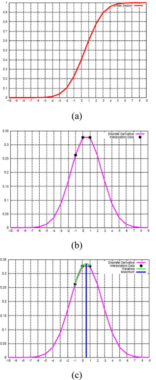
The sub-pixel edge detection using the interpolation method is as follows. First it extracts the edge at pixel level, and calculates the strength of the edge. Then, it extracts the edge at subpixel level using the parabolic or Gaussian modeling. This method has a precondition that the strength of the edge should be changed continuously and smoothly, also the surrounding area of maximum value of the edge can be modeled as parabolic or Gaussian modeling [14].
If the pixel level edge
As for the Gaussian modeling, we assume its function as follows:
When we substituted (-1,
Using (8), (9) and (10), equation (11) is obtained.
is the result of equation (8) subtracting (9) and dividing by (11). Here
Edge detection by sub-pixel interpolation takes less time because its calculation is relatively simple. But the strength of the edge does not change continuously and smoothly all the time, it may be changed rapidly. So it may be inaccurate to apply a parabolic or Gaussian modeling.
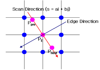
The parametric modeling begins with the idea that in the local area of images, the intensity value can be assumed as a continuous function [15]. It is impossible to express the changes of images’ intensity as a single continuous function, so we obtain a local continuous function called the facet model, with the surrounding pixels in a certain area. Using this continuous function, the intensity value of images at subpixel level can be obtained. The algorithm by the facet model is as follows.
As shown in the above algorithm, first we calculate the convolution
where -1≤
When the facet model can be defined as above, the direction of the edge can be obtained as follows.
Since
The weighting coefficients
Therefore, in order to obtain the facet model, we suggest not to obtain a polynomial coefficient directly, but to obtain the weighting coefficients
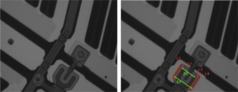
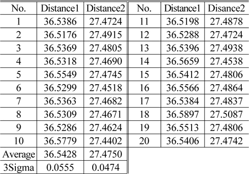
In this study, a sample pattern was produced in the process of TFT-LCD. The distance between the patterns was measured 20 times.
D1 : The distance between the L1 and L4 D2 : The distance between the L2 and L3
▪ Pixel level edge detection
[TABLE 1.] TFT CD measurement result using pixel level edge detection (unit: um)
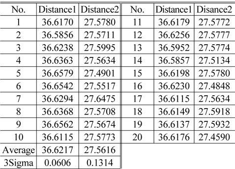
TFT CD measurement result using pixel level edge detection (unit: um)
▪ Subpixel level edge detection using parabolic interpolation
[TABLE 2.] TFT CD measurement result using parabolic interpolation (unit: um)

TFT CD measurement result using parabolic interpolation (unit: um)
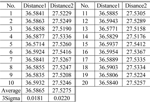
▪ Subpixel level edge detection using facet model
[TABLE 3.] TFT CD measurement result using facet model (unit: um)

TFT CD measurement result using facet model (unit: um)
In this study, we conducted research to develop a CD measurement algorithm of more stable and accurate TFT-LCD patterns, and the conclusion is as below.
1. We built a ring type of the reflected light optics for CD measurement and installed it in the stage. 2. For more accurate and high-speed measurement, we detected the edge’s accuracy of pixel level first, and detected the edge around the detected ones again of subpixel level.3. We used the first differential operator for the edge detection of pixel level. For the edge detection of subpixel accuracy, we modeled the detected edge filtered by LoG with the facet model, and calculated the local intensity continuous function, and obtained the zero-crossing with it.4. We compared the performances between the proposed subpixel edge detection algorithm and the existing interpolated subpixel edge algorithm, and pixel level edge detection. As a result, it is confirmed that the proposed algorithm can detect the edge most reliably and precisely.