The number of lens groups in modern zoom camera systems is increased above that of conventional systems in order to improve the speed of the auto focus with the high quality image. As a result, it is difficult to calculate zoom loci using the conventional analytic method, and even the recent one-step advanced numerical calculation method is not optimal because of the time-consuming problem generated by the iteration method. In this paper, in order to solve this problem, we suggest a new unified analytic method for zoom lens loci with finite object distance including infinite object distance. This method is induced by systematically analyzing various distances between the object and other groups including the first lens group, for various situations corresponding to zooming equations of the finite lens systems after using a spline interpolation for each lens group. And we confirm the justification of the new method by using various zoom lens examples. By using this method, we can easily and quickly obtain the zoom lens loci not only without any calculation process of iteration but also without any limit on the group number and the object distance in every zoom lens system.
An optical imaging system is generally classified by two types of finite and infinite object distances according to various applications [1]. The object distance is infinite for camera systems, while it is finite for microscopes and optical inspection systems. However, for certain camera systems, the optical systems have sometimes finite object distances, Such is the case for macro lenses [2]. Although a macro lens is classified as a single focus lens, the optical design method does not shows any difference compared to a conventional zoom lens design because two or more lens groups are generally used for focusing. When two or more lens groups are moved, it is called a floating system. Even in this case, the displacement of each lens group according to the focusing adjustment could be derived in the same way as the general zoom lens system. Of course, the displacement of each lens group determines the locus of the optical system. The result from this calculation is important in the manufacturing process for the cam components in zoom lens systems. In addition, there are optical systems with finite object distances that achieve a fixed magnification by moving the sub-groups along an optical axis, in spite of the variation in the object distance [3]. In particular, this type of system is called a multi-configurative optical system [3] because it does not follow the typical definition of a zoom lens [4]. Nevertheless, the multi-configurative optical system is also designed with from three to five discontinuous zoom configurations like an ordinary zoom lens system in order to improve the performance of the optical system. The displacement of each group needs to be precisely calculated for cam manufactures similar to other zoom lenses because the optical system consists of a variator, which prevents the variation of the lateral magnification, and a compensator, which compensates the variation of the image plane depending on the movement of the variator.
Therefore, in an optical system with finite object distance, it is necessary to calculate the zoom loci, similar to the conventional zoom lens, when more than two lens groups move. In the calculation of zoom equations for the zoom loci, the values of these loci can be obtained analytically according to the given constraint of an optical system [1]. This method derives the values of these equations analytically after classifying the optical systems according to constraints. However, the analytic method corresponding to each constraint is difficult to use practically and universally when the number of the group of the lenses is large, because every situation must calculated one by one. A numerical analysis method for the locus calculation has already been proposed as a way to solve all the constraints [5, 6]. Nevertheless, this method iterates the calculations by a Jacobian matrix differential equation simultaneously with the zoom equations and constraints. Therefore, this method is time-consuming, and the programming for the numerical method becomes very complicated when solving the simultaneous nonlinear equations of the zoom equation and its inverse matrix. In addition, because the convergence rate is becoming small as the absolute value of the determinant of the Jacobian matrix is converging to 0, the precision of zoom loci is rapidly reduced. Recently, although the new analytic method has been proposed in order to solve the problem, it is the method obtained by applying to a zoom lens for an optical system with infinite object distance, such as a camera lens [7].
In this paper, a new method using a zoom lens as an optical system with finite object distance, which is more powerful and effective in expanding compared to using the results from Reference [7] is proposed. In other words, the effectiveness of a unified analytic method for calculating the zoom locus, which is the non-iterative analytic calculations of the locus, is discussed for the unified zoom system, regardless of the number of lens groups and constraints, the distance from zoom lens to object, and format of the optical system such as a floating and multi-configurative optical system [8].
II. THE UNIFIED ANALYTIC METHOD OF CALCULATING LENS LOCI
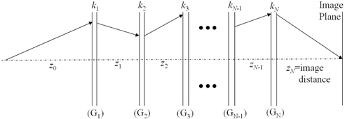
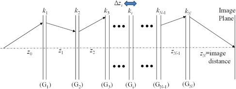
Figure 1 shows the optical layout of a finite object optical system with N groups in terms of the axial rays of the finite object. The zoom locus is derived by calculating the distance between groups in order to constrain image points to 0 on a paraxial image point at all times regardless of its location. Currently, the axial ray is needed to satisfy the given magnification and object distance, while the image height of the axial ray remains 0 on the paraxial image point.
Therefore, for the calculation of the zoom locus, the distance between groups must be obtained in order for the lateral magnification of the optical system to have the desired value with the image point of the axial ray fixed at 0 on the image plane. The distance between groups is virtually given by paraxial ray tracing about the axial ray. In such an optical system, paraxial ray tracing about an axial ray is expressed in terms of a Gaussian bracket [1].
where
Because the object distance is infinite regardless of the zoom configurations of the optical system, the object distance has an unknown variable value. However, the object distance is often given in optical systems with a finite object distance. The lens locus is the data that a mechanical designer of a camera is given from an optical system designer in order to design and manufacture CAM components after finishing the lens design. Meanwhile, the physical quantity that determines the field of view in an optical system with infinite object distance is the refracting power or focal length. However, magnification is the physical quantity that determines the optical system. Therefore, compared to the unknown parameter of the two types of optical systems in equal N groups, the number of the unknown parameters in an optical system with infinite object distance is N+1. This includes the focal length and number of intervals of each group. However, the total number of unknown parameters in an optical system with finite object distance is N+2 when the object distance is added. Therefore, the unknown parameters in equation (1) are
On the other hand, because the optical system is complicated, the constraints are not clearly given and only two variables can be unknown when calculating the two zoom equation. Figure 2 shows the optical layout when the i-th group is moved Δ
The
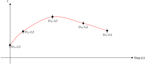
The distances of each group,
As shown in Fig. 3, each section of the curve can be expressed as a third-order polynomial similar to equation (3). This polynomial is continuous at the zoom position. If the 1st derivative is continuous, the equation (3) is satisfied. Because
If equation (3) is expressed in the matrix form, then equations (4), and (5) can be determined by solving the inverse matrix of equation (4) with the unknown parameters
For equation (3) - (5),
2.1. Case 1: The Case That the Object Distance Changes and the 1st Lens Group Moves
When the position of the 1st lens group and the object distance varies simultaneously, equation (2) can be expressed as
Where unknown parameters are the object distance
When
The numerator and denominator of equation (7) can be rewritten in terms of Δ
When equation (8) is rewritten in terms of Δ
Between the two solutions of Δ
2.2. Case 2: The Case That the Object Distance Changes and the Other Lens Group Moves
For Case 2, image distance (
where the unknown parameter is the compensating parameter Δ
Solving equation (10) simultaneously for
Similarly, the numerator and denominator of equation (11) can be rewritten for Δ
Even if equation (12) looks complicated, using the rules of algebraic equations yield a quadratic equation for Δ
As in Case 2, the lower absolute value for Δ
III. EXAMPLES OF CALCULATING LENS LOCI
The effectiveness of the unified analytic method, which has been previously described in session II, is verified by calculating the zoom locus for some of the optical systems with a finite object distance.
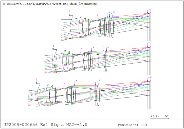
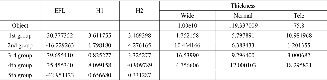
The first example of JP2008-020656[8] will be used to examine the usability of equations (7) and (9) of Case 1. This example is a type of optical system that moves both the 1st and 2nd groups. This optical system, a doublegauss type, was mainly used for the macro lens in the initial stage. It is easier to move than fix the 2nd group in order to make the lens aperture smaller, considering the size of the mount for the interchangeable lens. Figure 4 shows the optical layout of the 1st example of JP2008-020656, and Table 1 represents the specifications, such as the focal length for each group, the location of the principal point, and the distance between groups. In Table 1, the locus is calculated, assuming that the cover glass of image sensor and the optical low pass filter (OLPF) are located at the back of the 2nd group. It also assumes the total thickness of both the cover glass and the OLPF is 3 mm.
[TABLE 1.] The specifications for JP2008-020656

The specifications for JP2008-020656
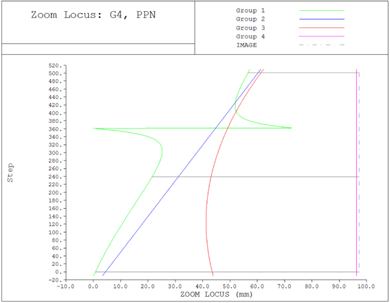
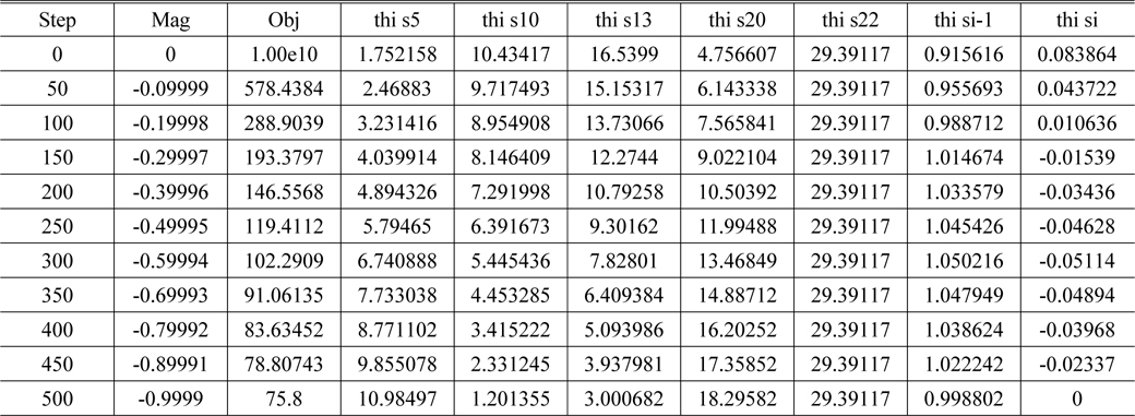
Table 2 and Fig. 5 are the result of the zoom locus calculation for JP2008-020656. The zoom locus is calculated by assuming that the 2nd group moves linearly. This is practical because of its advantage of the linear displacement for CAM manufacture. Because the main purpose is to verify the given equation of the locus calculation in Case 1, the zoom locus is not linearly calculated as a compensator at this point although it is possible to linearly calculate the 1st group.
The locus for US2010-0177407A1 determined by compensation of the 1st group for linearization of the 2nd group
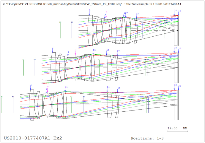
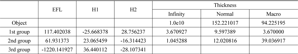
The groups in the 2nd example of US2010-0177407A1[9] are not fixed but movable. This is because it is designed to examine the convenience and accuracy of its usability for the zoom locus calculation by using equations (10) and (13) for Case 2. In this case, optical system must be brighter than JP2008-020656 due to the lower F-number, Sufficient optical performance can be obtained when it is possible to move the three groups, which are divided by the stop in its front and back. In this case, the group in the front of the stop is the 1st group, the one in the back of the stop is the 2nd group, and the one behind the 2nd group and the closest to the image plane is the 3rd group. Figure 6 displays the optical layout of US2010-0177407A1, and Table 3 shows the specifications, such as the focal lengths for each group, the location of the principal point, and the distance between groups.
[TABLE 3.] The specifications for US2010-0177407A1

The specifications for US2010-0177407A1
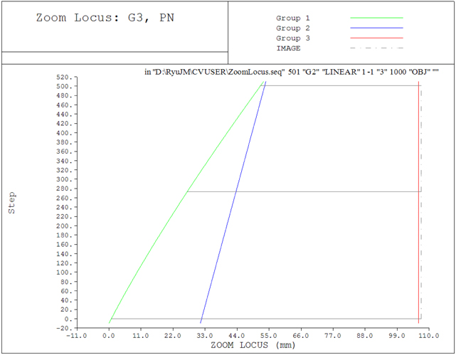
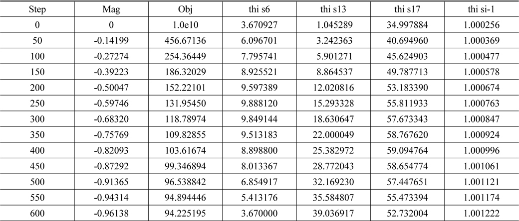
Table 4 shows the displacement of the 2nd group and the object distance. This represents the locus value for a non-linear magnification that depends on the rotation of the CAM and the given image distance. The magnification of this system is changed by 2nd-order polynomial

The locus for US2010-0177407A1 determined by compensation of the 1st group for magnification by given 2nd-order polynomial (y=ax2+bx)
For US2010-0177407A1, it is impossible to calculate the locus shown in Fig. 8, unlike Case 1. This is because when calculating the longitudinal sensitivity [10], the magnification of the 1st group becomes 1x in between the infinite zoom position and the middle zoom position. This results in a zero longitudinal sensitivity. Therefore, when it comes to calculating the zoom locus, the determination of whether the longitudinal sensitivity becomes 0 or not must be verified in advance. Similarly, the 3rd group is not adequate as a compensator because the maximum value is too low despite the longitudinal sensitivity of the 3rd group not being 0. Therefore, it cannot practically be used as a compensator.
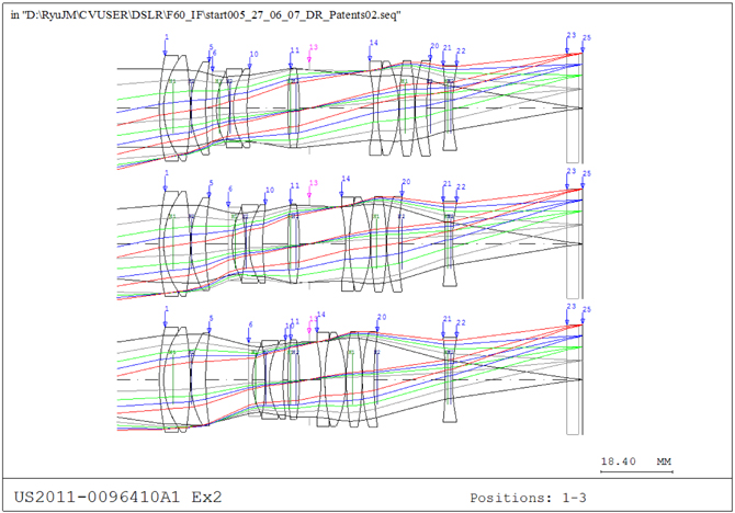
The effectiveness of Case 2 can be more clearly examined when there are more groups of the zoom optical system. US2011-0096410A1 [11] is a macro lens. This optical system uses the inner focus system where the entire length of the optical system is fixed while adjusting the focus. Therefore, this optical system is more advantageous to take a picture of a moving subject such as insects. However, extraordinary technology is required due to the larger sensitivity of the macro lens in the form of double-gauss. Figure 9 displays the optical layout of US2011-0096410A1, and Table 5 shows the specifications to calculate the locus.
[TABLE 5.] The specifications for US2011-0096410A1

The specifications for US2011-0096410A1
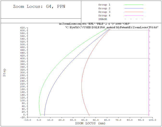
Table 6 and Fig. 10 are the result of the zoom calculation of the compensations for the displacement of the 4th group and the object distance assuming a linear magnification for US2011-0096410A1. In effect, Table 6 verifies the linear magnification for US2011-0096410A1.

The locus for US2011-0096410A1 determined by compensation of the 4th group for linearization of magnification
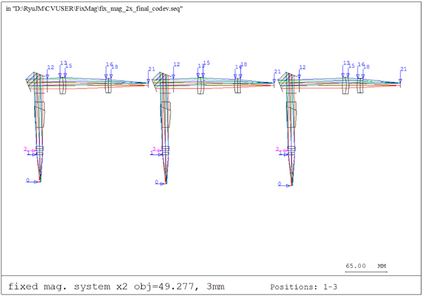
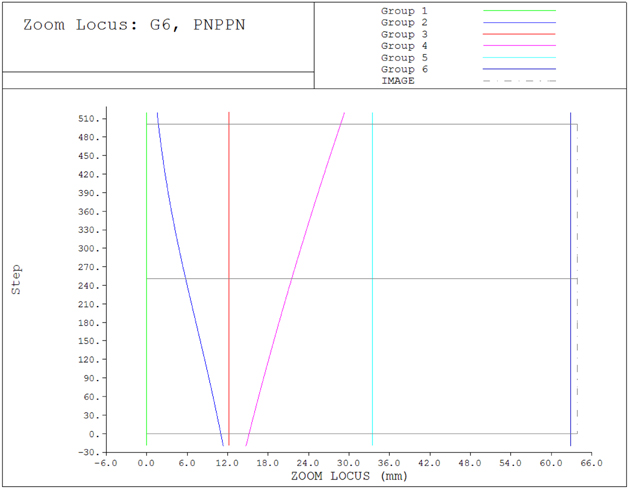
Lastly, the case of an optical system with a fixed magnification regardless of the changing object distance, which is classified into the multi-configurative optical system [7], is determined. Because the magnification for every zoom position is not zero, this optical system, as a device for lead frame inspection, has a finite object distance. The method introduced in section II can be used to calculate the locus for this optical system.
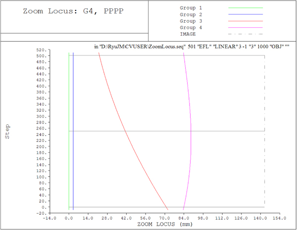
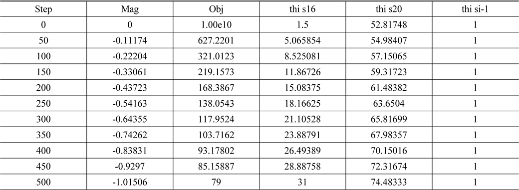
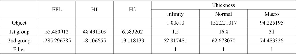
In the Reference [7], the specifications and the product design data are described in detail; thus, they are omitted at this point. Figure 11 displays the optical layout of this optical system, and Table 7 lists the focal length of each group, the location of principal point, and the distance between groups. The 1st group consists of a total of two lens groups. They are classified into 1-1 group that is comprised of one piece of a biconvex lens and 1-2 group that consists of two pieces of cemented lenses. The entire 1st group is fixed when the 2nd and 3rd groups move. Table 8 shows the locus table by the compensation of the 3rd group for fixed magnification, and Fig. 12 presents the locus for the example described in Reference [7].
[TABLE 7.] The specifications for the example in Reference [7]
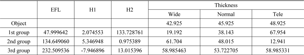
The specifications for the example in Reference [7]
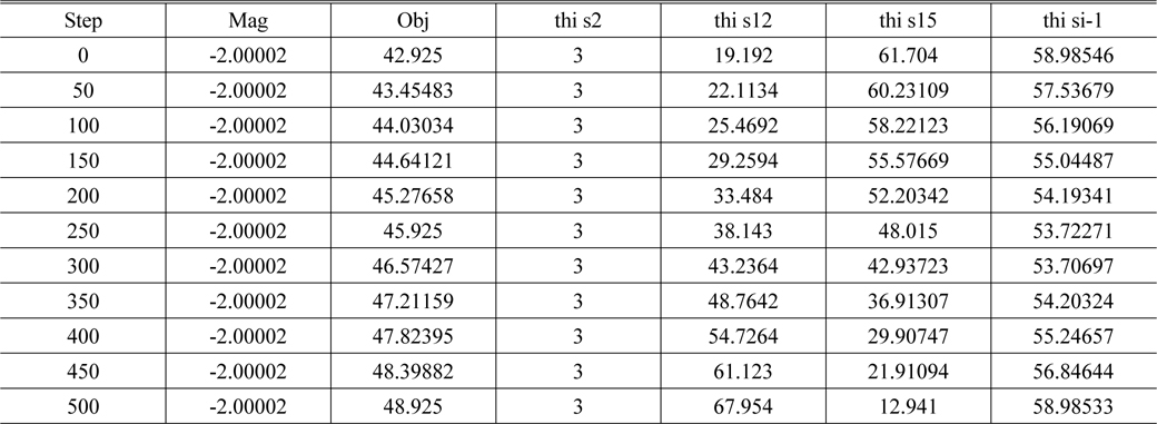
The locus for the example in Reference [7] determined by compensation of the 3rd group for fixed magnification
Similar to the procedures described above, various practical examples were verified using the unified analytic method of calculating a lens loci that adapts then Gaussian bracket method. This is derived from the examination of all zoom lens types and the multi-configurative optical system and a similar type of a zoom lens optical system for both case 1 and case 2. Consequently, the existing results correspond with those of Figs. 5, 7, 10, and 12 that are each calculated by adapting References 9 and 10 (about the general zoom lens), Reference 12 (about the macro lens with a number of groups), and Reference 7 (about multi-configurative optical system, a similar type of a zoom lens optical system).
There is a high demand for zoom optical systems with finite object distance, because it is widely used with macro lenses as a sub-part of interchangeable lenses and many optical inspection systems. Even though this optical system does not fit within the definition of a standard zoom lens, many groups still attempt to use this system as an optical system. Therefore, the displacement of each group should be calculated for each CAM build. As a result, the designing method is very analogous to that of a general zoom lens. Thus, the locus calculation is required for this optical system with finite object distance, too. Although the existing analytic and numerical method is known, our new method for the locus calculation is seriously needed because of the problems such as the complex process of obtaining the analytic value, waste of time for iterations, and calculation for the differential of the inverse matrix.
To achieve this, in this paper, an analytic method is proposed to show that the zoom loci can be obtained by moving the object distance and an added group, regardless of the number of groups. Imaging conditions need to be satisfied on the image plane for a given magnification and axial ray after interpolating the displacement of each group based on the data given in the initial optical design by a spline interpolation. This verifies that the desired locus can be easily obtained from various types of optical systems.
Various practical examples were verified by the unified analytic method of calculating lens loci that adapts the Gaussian bracket method, which is derived from the examination of all zoom lens types, multi-configurative optical systems, and a similar type of a zoom lens optical system in both Cases 1 and Cases 2. Consequently, the existing results corresponding with Figs. 5, 7, 10, and 12 are each calculated by adapting References 9 and 10 (about a general zoom lens), Reference 12 (about a macro lens with a number of groups), and Reference 7 (about a multi-configurative optical system, a similar type of a zoom lens optical system). Unlike the conventional zoom locus calculation method, which separately calculates the different kinds of groups for zoom lenses and the types of lenses, or adapting a numerical analysis from the results, this paper verifies the effectiveness of this new method by both deriving an analytic equation and adapting it to many cases successfully.


![Optical layout for the example in Reference [7].](http://oak.go.kr/repository/journal/13795/E1OSAB_2014_v18n2_134_f011.jpg)
![The specifications for the example in Reference [7]](http://oak.go.kr/repository/journal/13795/E1OSAB_2014_v18n2_134_t007.jpg)
![The locus for the example in Reference [7] determined by compensation of the 3rd group for fixed magnification](http://oak.go.kr/repository/journal/13795/E1OSAB_2014_v18n2_134_t008.jpg)
![Locus for the example in Reference [7].](http://oak.go.kr/repository/journal/13795/E1OSAB_2014_v18n2_134_f012.jpg)