The measurement and analysis of full-field strain distributions is very important in mechanical engineering, especially in the stress concentration problem in plastic and fracture mechanics. Conventionally, strains are measured by contact strain gauges and extensometers. The disadvantage of these two techniques can only provide the average strain of the local area and are not suitable for full-field deformation measurements [1]. A traditional strain distribution measurement is as follows: A grid is established on a sample surface before the deformation. We can measure the displacements of the grid after the deformation and analyze the strain distribution. The disadvantage of this method is that it is time consuming at analyzing the data. There are also precise measurement instruments, such as photoelasticity and electrical speckle pattern interferometers, which can be used to measure the surface strain field without contact [2-3]. But due to the expensive cost and the stability problem those methods cannot be widely used in scientific research and engineering.

A precise measurement of the surface strain distribution can be achieved with the help of the digital image correlation (DIC) technique (also known as the Digital Speckle Correlation Method). As compared to the special requirement of traditional optical measurements, digital image correlation is an easy and cheap method because it takes advantage of the speckle pattern on the specimen surface and only digital images taken by CCD/CMOS camera are processed. The DIC technique is predicated on the maximization of a correlation coefficient that is determined by examining the pixel intensity array subsets of two or more corresponding images and extracting the deformation shape function that relates the images to each other [4]. In a general way, once the displacements at the entire region of interest (ROI) in the deformed image have been calculated, the strains are calculated using this displacement field by using numerical differentiation techniques [5]. Although the relationship between the strain and displacement can be described as a numerical differentiation process in mathematical theory, unfortunately, the numerical differentiation is considered as an unstable and risky operation [6], because it can amplify the noise contained in the computed displacement. Therefore, the resultant strains are untrustworthy if they are calculated by directly differentiating the estimated noisy displacements [7].

A more practical technique for strain estimation is the pointwise local least-squares fitting technique used and advocated by Wattrisse [8] and Pan [9]. Wattrisse [8] implemented a local least-squares method to estimate the strains from the discrete and noisy displacement fields computed by the DIC to analyze the strain localization phenomena during the tension of thin flat steel samples. A similar technique was also used by Pan [9] with a simpler and more effective data processing technique for the calculation of strains for the points located at the image boundary, holes, cracks and the other discontinuity areas. Xiang [10] used the moving least-squares (MLS) method to smooth the displacement field followed by a numerical differentiation of the smoothed displacement field to get the strain fields. Different from above pointwise algorithms, the Q4-DIC developed by Besnard [11] and the finite element method proposed by Sun [12] can be classified as a continuum method, in which the surface deformation of the sample is measured throughout the entire image area. These techniques ensure the displacement continuity among pixel points. However, reported results showed that these two methods seem not to provide higher displacement measurement accuracy than gradient-based algorithms. Nevertheless, they can provide new ideas for strain measurement. After obtaining the displacements of points in the region of interest, the finite element method (FEM) is used to estimate continuous strain fields from the continuous displacement fields.

In this study, a two-step DIC strain measurement method is presented. In the first step, the gradient-based subpixel technique is used to search the displacement of a region of interest of the sample, and then the strain can be obtained by utilizing the finite element method in the second step. Both simulation and experiment are carried out to verify the accuracy of this method.

Digital Image Correlation (DIC) is based on a comparison between two digital images of a sample surface captured at two different levels of loading. The discrete pixels of these digital images and their grey values for intensity were recorded and transferred as a two-dimensional array. Under the assumption that there is a one-to-one correspondence on the intensity pattern of two images taken before and after deformation, one could deduce the deformation information from comparison.

In this study, in order to reduce the noise from the CMOS camera and the backlight, a 2D adaptive noiseremoval smoothing technique was applied to the obtained digital image. This function could smooth the grey level of a pixel according to the average value and standard variation of its neighbor pixels. The average value could be obtained as follow.

The considered region is denoted as η that consists of M×N pixels, and n₁, n₂ represents a point of this region. The original grey level is represented as I_a. The standard variance is calculated as

Then the smoothed grey level could be obtained as

where ν² is the average standard variance of all regions.

After the smoothing treatment, these two smoothed images, which characterize the original and deformed surfaces of a material subjected to a known loading, were used to evaluate the deformation. A square reference subset of (2M + 1) >× (2M + 1) pixels centered at the point (x₀, y₀) is arbitrarily chosen from the reference image and a reference point (x, y) is selected from this subset, the position (x′, y′) of the reference point after the deformation increment could be described as

where u₀ and v₀ are the integral pixel displacements in the x and y directions, which can be accurately determined with ease and are assumed as known values; ∆u and ∆v are the corresponding sub-pixel displacements in the x and y directions, respectively. The whole subset is assumed to have the same displacements. Under this assumption, both the subset and the deformation increment should be small.

A sum-squared difference (SSD) correlation function is used for deriving a theoretical model of the displacement measurement accuracy of DIC. The SSD correlation function is defined as [11]

where f(x, y) is the grayscale intensity value at point (x, y) of the reference image, and g(x′, y′) is the grayscale intensity value at point of the deformed image.

After neglecting the high-order terms, the first-order Taylor expansions of g(x′, y′) yields

where g_x and g_y are the first-order derivatives of grayscale intensities, and in this study they are calculated by central difference of neighboring points in the x and y directions, respectively.

Minimization of the SSD correlation function would provide the best estimate of the desired sub-pixel displacements ∆u and ∆v. Thus we have

The solution of Eq. (7) can be expressed in the following closed form

Once the location of the target subset in the deformed image is found, the displacement components of the reference and target subset centers can be determined. More details of the error estimation of the DIC technique can be found in Ref. [13].

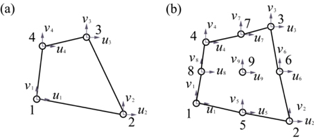
After obtaining the displacements of points in a prescribed region, the concept of four-node quadrilateral (Q4) finite element as shown in Fig. 1(a) is utilized to calculate the strains in the region defined by four node points. Consider an arbitrary point with the coordinates x and y in this region, its displacements along the x and y direction are

where a_i and b_i are constants that could be obtained from the displacements of the four node points. Then the strains in this region could be calculated by the following equations

where ε_xx and ε_yy are normal strains and γ_xy is the shear strain. In addition to the four-node quadrilateral (Q4) finite element, the concept of nine-node quadrilateral (Q9) finite element as shown in Fig. 1(b) is also used to calculate the strain from the displacement information. Then, the displacements of an arbitrary point in the element could be described as

where a_i and b_i are constants that could be obtained from the displacements of the eight node points. Then the strains in this region could be calculated by the following equations

To verify the efficiency of the proposed method, a typical tension deformation with and without noise are designed to explore the precision and noise-robustness of the method. Then, a real tension deformation with DIC is processed to validate the ability of the real data.

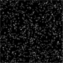
In the precision comparison experiments, the speckle images before and after deformation are generated using the algorithm developed by Zhou [14]. The simulated image is 512×512 pixels with 1200 speckles, each 4 pixels in size, as shown in Fig. 2. The subset is 41×41 pixels, displacement fields are calculated using the gradient-based method.

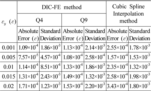
To test the precision of the DIC-FE strain measurement method, the experimental results are compared with the results obtained by the cubic spline interpolation method [15], as shown in Table 1. All of the results are the average of 20 independent experiments on the center point.

In the simulated tension deformation experiment, the displacement gradient (strain) ε_y is 0.001~0.02. Table 1 shows the absolute error and standard deviation of the central points obtained by the proposed and cubic spline interpolation methods, respectively. The comparisons show the strain precision of the proposed method being better than 2×10^-4ε, higher than that of the cubic spline interpolation method. Both Q4 and Q9 types of the DIC-FE method have very close results. The comparisons demonstrate that the proposed method can achieve a high accuracy strain measurement.

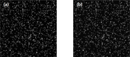
To explore noise-robustness of the proposed method, two Gaussian noises (with means of 0 and variance of 0.2 and 0.5) are added to the same simulated image in “Simulation without noise”. Fig. 3 shows the noise-added simulated speckle images (with variance of 0.2 and 0.5) before deformation. The subset is also 41×41 pixels.

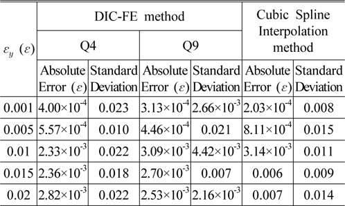
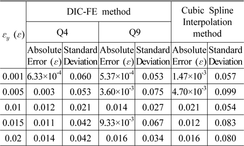
Tables 2 and 3 show the absolute error and standard deviation of the central points of 20 simulated images obtained by the proposed and interpolation methods. The comparisons show that both can get the relative proper results and the precisions of the proposed and interpolation methods decline with the increase of noise. It can been seen from Table 3 that the precision of the proposed method is better than 0.015, a little higher than that of the cubic spline interpolation method. For the lower noise level, the precision showed in Table 2 is higher Table 3.

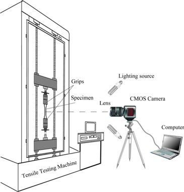
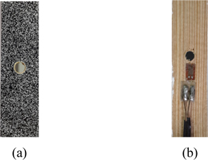
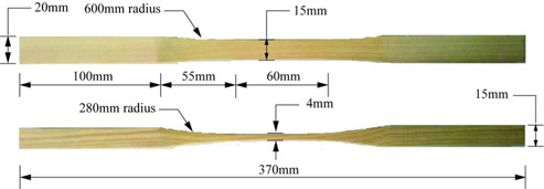
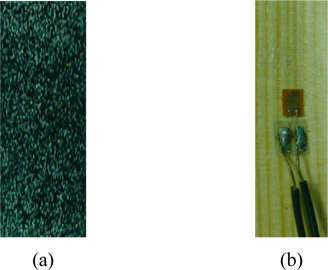
To evaluate the effectiveness of the proposed DIC-FE strain measurement method in real data processing, dogbone specimens of Dahurian Larch wood were used in a uniaxial tensile test (Fig. 4). The surface of the specimen was sprayed uniformly with white paint on the region of interest, and then black paint was sprayed randomly (Fig. 5(a)). To have reference strain values, a strain gauge was attached at the back surface of the specimen (Fig. 5(b)). Preparation of the testing equipment occurs after the speckle pattern application to produce a testing configuration as shown in Figure 6. The uniaxial tensile testing was conducted on a tensile testing machine and the crosshead loading rate was 3 mm/min. During the testing process, two LED lights were used to shine on the specimen, and the image was taken every 10 seconds. The digital camera used was a CMOS industrial camera with the resolution of 1024×1280 pixels, focal length 8 mm, and f /1.8. The image magnification was about 0.04549 mm/pixel.

Strains at rectangle speckle cells with the coordinate x from 590 to 690 pixels and y from 490 to 540 pixels with an interval of 5 pixels are obtained by the DIC-FE method. The strain gauge was applied at the same zone of the back surface of the specimen to obtain the strain information for comparison with those obtained by the present DIC-FE method. When both the four-node element and the nine-node element are used, the comparison is shown in Fig. 7. It is evident that the present results have good agreement with those from the strain gauge, and the two types of elements have very close results. In considering the calculation time, the present DIC-FE method with fournode element should be a good choice.

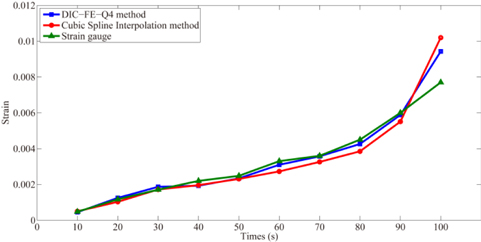
In this testing, strain gauge was also applied to obtain the reference strain values of a specimen with a hole (Fig. 8). In this case, the strains around a hole have a high gradient. Hence, this specimen could represent the application of the present method to a high strain gradient region.

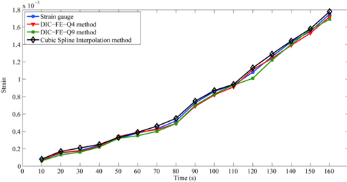
As shown in Fig. 9, the present method with four-node element could obtain reasonable strains in the high strain gradient region as compared to the strain gauge and spline method.

From the above analysis, it is concluded that the proposed DIC-FE-4Q strain measurement method can be used in experimental cases including strain deformation, and it is able to obtain nearly the same results and calculating time when compared with the cubic spline interpolation method.

This article introduces a finite element based strain measurement algorithm to DIC computation, a two-step DIC is presented. In the first step, the gradient-based sub-pixels technique is used to search the displacement of a region of interest of the specimen, and then the strain can be obtained by utilizing the finite element method in the second step. Simulated results show that its precision is a little higher than that of the cubic spline interpolation method. Finally, this method is used in the uniaxial tensile testing for Dahurian Larch wood specimens with artificial painting on the surface, and the obtained strain values are close to the results obtained from the strain gauge. When this method is applied to measure the strain of a specimen with a hole, it shows that this DIC method with four-node element could obtain correct strains even in the high strain gradient region.