Spatial distribution of individual trees in an overcrowded population is initially random, and then becomes uniform as trees grow (Kenkel 1988). Because plants lack the ability to migrate, this uniform spatial distribution arises as a consequence of tree death. The dead trees are smaller individuals dying as a result of interactions with other trees (Silvertown and Charlesworth 2001, Gurevitch et al. 2006).

Interactions between animals are easily observed. For example, competitive interactions associated with territorial defense are readily evidenced by aggressive behavior towards other animals. Because plants cannot move on their own, their interactions are less obvious; however, a dataset of measured diameter at breast heights (DBHs) and/or heights can be generated to estimate the interaction. In this study, we used such a dataset to detect competitive interaction manifested by lower-than-usual growth rates and/or deaths of trees. Because lower growth rates and/or death may arise from factors such as disease in addition to disturbance, however, plant population mortality is difficult to predict.

Mithen et al. (1984) have reported that individuals of the herb Lapsana communis with small “available area” are likely to die, but it is unclear whether this observation is relevant to tree species. Bigler et al. (2004) found evidence of relatively low late-stage growth rates in growth patterns from dead trees, although those authors focused on Abies alba, a shade-tolerant (Rolland 1993), late-succession- stage tree (Kienast and Kuhn 1989).

In the study reported here, we used data collected over a 37-year period to predict Pinus densiflora mortality based on DBH and available area. The analyzed data comprised a long-term dataset of DBHs recorded from two study plots of naturally established P. densiflora, a shade-intolerant pioneer species (Han et al. 2003), and position data (xy coordinates) of all the individual trees in one of the two plots.

The study site is located on the campus of the Sugadaira Montane Research Center of Tsukuba University (SMRCT), Nagano Prefecture, Japan (36°31' N, 138°20' E) at 1,320 m above sea level. The study site is on a southwest- facing slope with an incline of 5°. According to the records of the SMRCT from 1971 until 2000, mean annual temperature is 6.5°C and mean annual precipitation is 1,190 mm. The site is snow-covered each year from November to April, with a mean snow depth cover of 48 cm in January, 74 cm in February, and 64 cm in March (Japan Meteorological Agency 2001). The top soil is derived from the Quaternary volcanic ash of Mt. Azumaya (Suzuki, personal communication). Before the campus was established in 1934, the land was an abandoned farm field or meadow. Monitoring was carried out in a P. densiflora stand that developed from a Miscanthus sinensis grassland by secondary succession. Permanent plot A (20 m × 20 m quadrat) was established in 1973 at the experimental site, and permanent plot B (40 m × 20 m) was set up in 1977. DBHs of the canopy trees in Plot A were measured in 1973, and then annually from 1976 to 2010; the same measurements were made annually in Plot B from 1977 to 2010. Hayashi (personal communication) measured positions (xy coordinates) of all individuals in Plot A in 1973.

To evaluate spatial distribution of trees in Plot A, we used Ripley’s K function (Kenkel 1988). The K function is defined as follows:

where A is the area of the plot, n is the number of individual trees, f(i, j, r) is a function equal to 1 if the distance between trees i and j is equal or smaller than r, and 0 otherwise, w(i, j) is an edge-correction function, and r is a distance variable (Fortin and Dale 2005). We adopted the Ohser-Stoyan edge correction factor (Li and Zhang 2007), with w(i, j) accordingly defined as follows:

where a and b are plot length and width, and x is the distance between trees i and j. The K function was converted into an L function as follows:

If the distribution is completely random, L(r) is zero. To test the null hypothesis of spatial randomness, we computed a 95% confidence interval using the Monte Carlo method with 500 simulations. (Diggle 1983, Shimatani 2001).

Calculation of available area—a polygon—of a tree was conducted by counting the number of points that were closer to that tree than to any other trees in the plot (Mithen et al. 1984). We applied a toroidal edge correction when calculating polygonal areas (Cherubini et al. 2002).

To compare DBHs among different years, we converted them into relative DBHs (rDBHs) by dividing each DBH by the annual mean DBH (Luo and Chen 2011). We obtained relative areas (rAREAs) in a similar fashion, dividing each available area by the mean available area for that year.

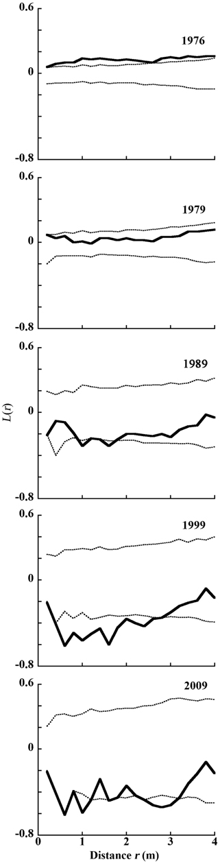
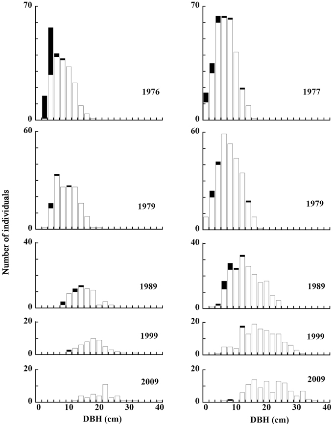
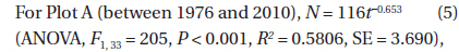
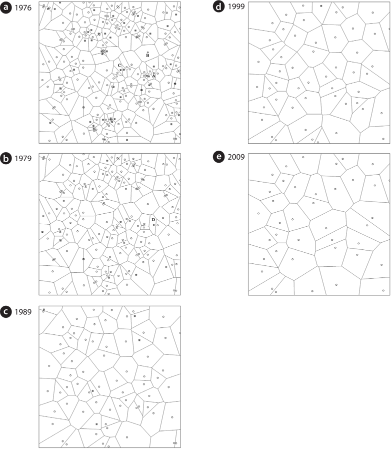
The distribution of living and dead individual trees from 1976 to 2009 in 20 m × 20 m Plot A is shown in Fig. 1. As the number of trees decreased, their available areas became larger (Fig. 1a-1e). During the monitored period, the distribution pattern was clumped at first (in 1976). In 1979, it became random, and after 1989 was uniform (Fig. 2) (Kenkel 1988). DBH histograms of living and dead individuals in Plot A from 1976 to 2009 and in Plot B from 1977 to 2009 are shown in Fig. 3. DBHs of dead individuals (Plot A between 1976 and 1999, and Plot B between 1977 and 1989) were mainly small.

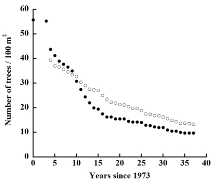
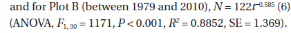
The decline in tree density in plots A and B from 1973 to 2010 (Fig. 4) followed an exponential decay function. For Plot A, the decay function is:

where N(t) is density (trees/100 m²) of the plot and t is the number of years since 1973 (ANOVA F_{1, 34} = 277, P < 0.00001, R² = 0.6734, SE = 22.29). The decline in density of Plot B followed a similar equation, with the coefficient and power equal to 43.83 and –0.0338, respectively (ANOVA, F_{1, 32} = 3,562, P < 0.001, R² = 0.9419, SE = 0.7417).

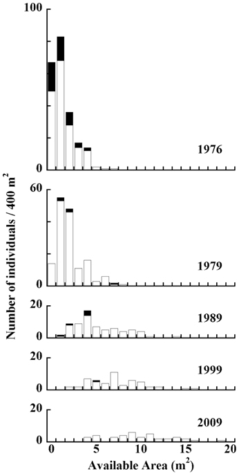
An available-area histogram of living and dead individuals in Plot A from 1977 to 2010 is displayed in Fig. 5. Between 1976 and 1989, we observed a strong tendency for trees with smaller available areas to have died. Between 1999 and 2009, there was a slight tendency for trees with smaller available areas to have died.

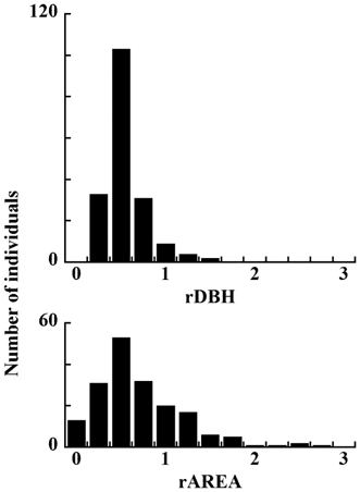
Histograms of rDBH and rAREA of dead individuals are shown in Fig. 6. Although they have the same modal values, the range of rAREA is wider than that of rDBH. This figure suggests that small rDBH had a stronger effect on tree mortality.

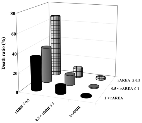
Small rDBH had a stronger effect on tree mortality than small rAREA (Fig. 7). Moreover, trees having both rDBH and rAREA not more than 0.5 had the highest mortality levels, while trees having rDBH and rAREA more than 1 had the lowest (Fig. 7).

Based on our data, the density N (individuals / 100 m²) of plots A and B can be estimated from t (years since 1972) as follows:

These two equations are of the form

Differentiating equation (7) with respect to t yields the following equation:

The left side of equation (8) is the probability of death at time t, and is proportional to the density N raised to the power of 1/b. The value of 1/b is greater than 0, indicating that density-dependent death is occurring in the studied populations. The spatial dispersion of individual P. densiflora trees changed from a random to a regular pattern over the course of the monitored period; this also suggests the occurrence of density-dependent mortality (Kenkel 1988, Miyata 1989, Kenkel et al. 1997).

As trees age, they die, and their available area becomes associated with that of adjacent living trees. Because the surviving trees cannot grow or extend woody branches into newly acquired available areas, some trees that die may be surrounded by relatively large available areas. A strong relationship was therefore not observed between smaller rAREA and tree mortality. On the other hand, an allometric relationship exists between DBH and tree height (Kato and Hayashi 2003), with individuals having smaller rDBHs typically characterized by smaller tree heights. Because P. densiflora is a shade-intolerant species (Han et al. 2003), shorter individuals have greater difficulty acquiring sunlight, leading to death.

During establishment period of naturally germinated P. densiflora populations, DBHs increased while number of individuals in the populations decreased. During self-thinning phase, density-dependent mortality occurred. The spatial dispersion of individual P. densiflora trees changed from a random to a regular pattern over the course of the monitored period. Smaller rDBH has a stronger influence on tree mortality than does smaller rAREA.