Infrared optical systems are operated at low temperature and vacuum (LT-V) condition to minimize thermal noise. In general, the manufacture, assembly, and alignment of optical systems are performed at room temperature and non-vacuum (RT-NV) condition. If the temperature and pressure conditions alter, the physical changes of optical and opto-mechanical parts occur (Kaneda et al. 2005, Leviton et al. 2005), and this drives the optical performance variation. For visible light optical systems that are operated at RT-NV condition, the tasks of alignment and performance measurement after measurement are also performed at RT-NV condition, and thus the alignment process is intuitive (Kim et al. 2005, Liu et al. 2005, Kim et al. 2007, Kim et al. 2009). However, for infrared optical systems that are operated at LT-V condition, assembly is performed at RT-NV condition whereas measurement is performed at LT-V condition, and thus the burdens of time and cost are incurred in regard to repeatedly changing the temperature and pressure.

The ‘no adjustment’ philosophy was devised to minimize the process of performance measurement after assembly. In this philosophy, assembly and alignment are performed within a mechanical tolerance range without optical measurement at RT-NV condition, and the optical performance can be implemented without a separate adjustment when it is changed to LT-V condition (Rio et al. 1998, Perrin et al. 2002, Glazenborg-Kluttig et al. 2003, Navarro et al. 2008). In order to employ the philosophy, the precise tolerance analysis of parts and the selection of appropriate materials are essential, and the precise manufacture of parts is required.

The systems that utilized the ‘no adjustment’ philosophy include MIDI (Perrin et al. 2002, Glazenborg-Kluttig et al. 2003), VISIR (Rio et al. 1998), and MIRI of JWST (Navarro et al. 2008). However, for MIDI and VISIR, opto-mechanical parts were precisely manufactured, but alignment was performed while moving the mirror or optical system at room temperature. Thus, the philosophy at those applications was partly applied. As for MIRI, precise manufacture and assembly were performed through the tolerance analysis using sensitivity analysis, and it was found to be within the tolerance by the measurement of the optical performance at operating temperature. However, the process of predicting or measuring the optical performance, which can be measured in assembly and alignment processes, in advance was not performed.

Besides the application of the ‘no adjustment’ philosophy, there are various methods for the effective assembly, alignment, and performance prediction of infrared optical systems that are operated in low temperature and vacuum environments. As for NIRSpec, optical alignment was attempted by comparing the predicted wavefront error (WFE) obtained by simulating the mirror plane and optical path, with the actual measured value (Taccola et al. 2008), but similar to MIRI, only the optical performance at operating temperature was considered. The planck reflector, which is installed at the PLANCK satellite, is also an optical part that is used at low temperature, but the surface figure error (SFE) was used as the optical measurement index (Roose et al. 2003). The Spectral and Photometric Imaging Receiver (SPIRE), which is used in the Herschel satellite, is also a spectrograph that is operated at low temperature, but for the assembly and alignment, a method, which aligns the cold stop of the spectrograph and the exit pupil of the telescope at which the spectrograph is installed, was used, and for the optical performance test, the Hartmann test was used (Dohlen et al. 2004). In general, for the performance measurement experiment of the Volume Phase Holographic Gratings (VPHGs) that are used in low-temperature nearinfrared optical systems (Insausti et al. 2008), the optical performance measurement of the Near Infrared Camera (NIC) that is installed at JWST (Ryder et al. 2008), and the optical performance experiment of optical systems that are made of SiC which is commonly used for the weight reduction of telescopes (Suganuma et al. 2010), WFE was measured through direct experiment without a simulation process. However, these methods predicted and tested the optical performance at operating temperature, but it was not that the assembly and alignment processes were performed while quantitatively predicting the performance at room temperature.

As stated above, for both when the ‘no adjustment’ philosophy was applied and when it was not applied, there has been no case that predicted the changes of optical performance at each step depending on the changes in temperature and pressure, and tested them at room temperature and at operating temperature. In this study, for the optical performance prediction experiment depending on the changes in temperature and pressure, the input relay optics (IO) module of the Immersion GRating INfrared Spectrograph (IGRINS) which is a silicon immersion grating infrared spectrograph for observing near-infrared region was used.

IGRINS is a near-infrared spectrograph, which has a high spectral resolution of R=40000 using a small-sized spectrograph that has been manufactured using silicon immersion gratings, and it was designed based on the ‘no adjustment’ philosophy (Lee et al. 2011). The IO module is one of the front end optical systems of IGRINS, which send the incident light (f/8) to f/10, and the module was designed so that it could have a focal plane of 2’x2’, the maximum required value during interferometer measurement could be 0.33 wv rms WFE, and the RMS spot radius requirement could be less than 25.7 μm (Jaffe et al. 2011, Lee 2012).

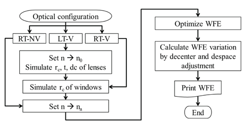
WFE was used as the index for optical performance prediction because it is easy to measure and the change of a value depending on the change in performance is very sensitive, which makes it appropriate for the optical performance prediction and testing factor. For the disagreement between the simulated and the experimental values, the degree of disagreement was improved by developing an adaptive fitting line so that the simulated values could be more precisely predicted. In Chapter 2, the method for predicting WFE at RT-NV, RT-V, and LT-V conditions was introduced; and in Chapter 3, the experiment process was described. In Chapter 4, the results and conclusion were summarized.

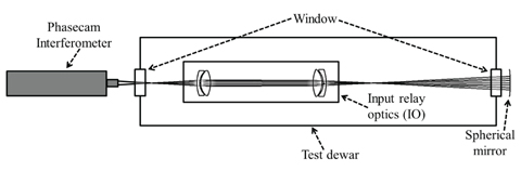
Fig. 1 shows the layouts of the simulation and the experiment, including the IO module. It is a path where the light (632.8 nm wavelength) from the interferometer (Phasecam 5030) forms the first focal point before entering the IO module, forms the second focal point after passing through the IO module that consists of four lenses, and then returns to the interferometer as it is reflected by a spherical mirror. For the test dewar used in the experiment, a total of two windows were installed, one on each side of the dewar.

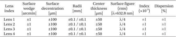
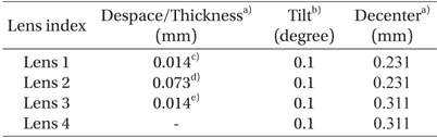
The wavelength used by IGRINS is the infrared band, but during measurement, the laser wavelength of the interferometer is the visible light region. Thus, the wavelength, which was applied to the simulation, was set to be identical to that of the interferometer. For the lenses of the IO module, the lenses at the front and at the back were made of S-FTM16, and the two lenses in the middle were made of CaF2. As the transition from RT-NV to RT-V is the transition from atmospheric condition to vacuum condition, the refractive index (n) and the curvature of the test dewar window change; and in the case of the transition to LT-V, the curvature and thickness of the lenses and the height of the optical axis change depending on the temperature variation. The alterations in the refractive indices of the lenses were applied by inputting the Sellmeier 1 formula coefficient (Sellmeier 1871, Radiant Zemax LLC 2013). Also, the manufacturing tolerances of the lenses are shown in Table 1 (Lee 2011).

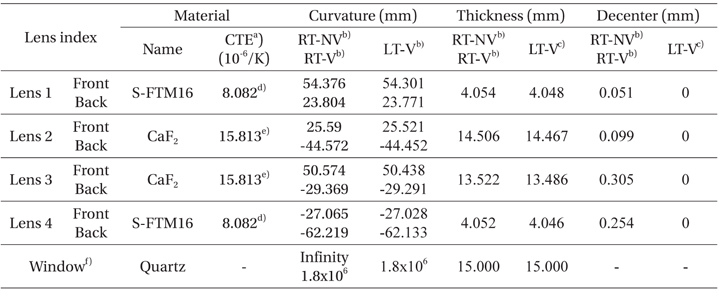
Table 2 summarizes the changes in the curvature and thickness of the lenses and the height of the optical axis depending on the change of condition. For the lens specification, the values at the RT-NV and RT-V conditions were the values provided by the lens manufacturer, and the values at the LT-V condition were the values calculated using the provided values and the thermal expansion coefficients that correspond to each material. For the refractive indices in air (n_a=1.000000) and vacuum (n₀=0.999728), the values provided by ZEMAX (Radiant Zemax LLC 2013) were applied. For the curvature of the window, the value, which simulated vacuum condition using Solidworks (ver. 2011 SP0), was applied to ZEMAX. The thickness was assumed as a constant because it does not affect optical performance. Table 3 summarizes the decenter, despace, and tilt, due to the changes of the opto-mechanical parts, at which the lenses were installed, depending on temperature. As all the opto-mechanical parts were made of Aluminum 6061- T6, the calculation was carried out by applying the same thermal expansion rate (Aluminum 6061-T6: 23.4x10^-6 /K; Marquardt et al. 2000, NIST 2013, Aalco 2013). For all the values, the LT-V condition was used as the standard, and the amount of change at room temperature relative to the LT-V condition was recorded.

Because of the differences in thermal expansion rates, the barrel, which was made of Aluminum 6061-T6, had a larger change in length due to temperature change, than the lenses, which were optical parts that were made of S-FTM16 and CaF₂. Thus, for the RT-NV condition, the expansion of the barrel was larger than that of the lenses, and there existed extra space between the lenses and the barrel within the IO module. However, it was difficult to directly measure the positions of the lenses that were in contact with the mount. Thus, the positions of the lenses (despace, decenter, and tilt) were set as variables, and optimization was performed using a default merit function. When the positions of the lenses, which were obtained from the optimization, exceeded the given tolerance range (despace: ±0.1 mm, decenter: ±0.15 mm, and tilt: ±0.1°; Lee 2011), the variables were fixed at the tolerance values, and optimization was performed again.

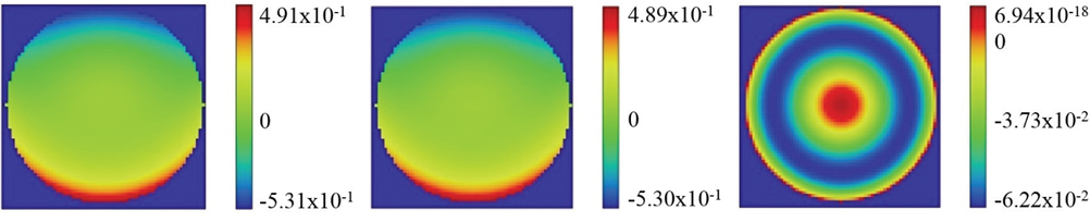
Fig. 3 shows the simulation results of WFE that was optimized at each condition through the above process. The optimal WFE values at each condition were 0.1873 λ root mean square (rms) at the RT-NV condition (Fig. 3a), 0.1868 λ rms at the RT-V condition (Fig. 3b), and 0.0182 λ rms at the LT-V condition (Fig. 3c). For the RT-NV and RT-V conditions excluding the LT-V condition, concentric circle shapes were not observed, which indicated that the alignment of the optical axis from the lenses to the spherical mirror was not appropriate. The maximum permitted WFE value of the IO was 0.33 waves (Lee 2012), and it was found that the simulation results shown in Fig. 3 did not exceed the allowable range.

As for the simulation of adjusting the position of the spherical mirror, the decenter was adjusted at ±0.15, ±0.2, and ±0.3 mm intervals, and the despace was adjusted at ±0.1, ±0.3, ±0.5 mm intervals, based on the tolerance range of the IO module, and the resultant changes in WFE were obtained. Section 3.2 shows the simulation results, along with the results of the experiment.

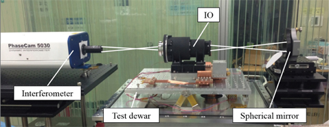
Fig. 4 shows the experimental setup that consists of the interferometer, IO module, spherical reflector, and test dewar. WFE was measured after the spherical mirror was adjusted so that the number of interference fringes could be the smallest. The WFE measured at that moment was the optimal WFE value for the RT-NV condition. For the RT-V and LT-V conditions, alignment was also performed while precisely adjusting the spherical mirror stage.

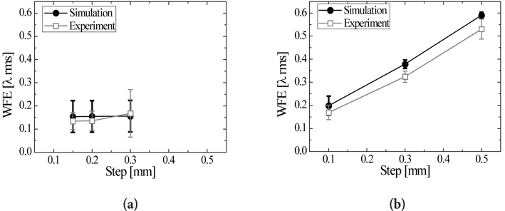
Through the X-, Y-, and Z-axis adjustment using the spherical mirror stage, the changes of WFE depending on the changes in despace and decenter were measured at three steps for each axis; and through the simulation and experiment, the optical performance of the IO module of IGRINS was measured. The optimal WFE at each condition depending on temperature and pressure was measured, and the resulting pattern of WFE was measured at each step at three conditions (RT-NV, RT-V, and LT-V) by adjusting the coordinate of the spherical mirror within specific intervals. Fig. 5 shows the obtained data. For the error bar, the standard deviation was applied. The IO was manufactured based on the ‘no adjustment’ philosophy, but as shown by the results, the simulated and the experimental values showed difference. Fig. 5a shows the results in which the X-axis and the Y-axis were adjusted independently or together, and Fig. 5b shows the results in which the Z-axis was adjusted (e.g., Z-axis independent adjustment, X-Z-axis linked adjustment, Y-Z-axis linked adjustment, and X-Y-Z-axis linked adjustment). For the X-axis and the Y-axis, if they are adjusted more than 0.3 mm in the experiment, fringes move outside the measurement screen during interferometer measurement. Thus, unlike the Z-axis, the maximum adjustment was set to 0.3 mm.

For the LT-V condition, the WFE value was very small (~0.018 λ rms WFE), and the amount of change due to the decenter (x and y direction movement) was also very small (~0.019 λ rms WFE) because the optimal optical performance, which can be implemented by an infrared optical system in simulation, was implemented. However, for the RT-NV and RT-V conditions, the decenter tolerance was small because the optical performance before the decenter was severe (~0.186 λ rms WFE), and thus the optical performance after the decenter was also high (0.187~0.189 λ rms WFE). Therefore, when the data for the RT-NV, RT-V, and LT-V conditions were presented together at a single step, as shown in Fig. 5, the difference between the minimum and maximum values was about 0.17 λ rms WFE, and the standard deviation of the data was large as shown in Fig. 5a.

As for the despace (z direction movement), the optical performance for the LT-V condition was 0.114~0.116 λ rms WFE at the 0.1 mm step, while the optical performances for the RT-NV and RT-V conditions were 0.213~0.224 λ rms WFE at the same step. The difference between the minimum and maximum quantities was about 0.11 λ rms WFE, and the standard deviation of the data in Fig. 5b was similar to that in Fig. 5a. However, at the 0.3 mm and 0.5 mm steps, the optical performance for the LT-V condition was 0.341~ 0.344 λ rms WFE and 0.568~0.572 λ rms WFE, respectively; and the optical performances for the RT-NV and RT-V conditions were 0.377 ~ 0.396 λ rms WFE and 0.579~0.609 λ rms WFE. The differences between the minimum and maximum values were about 0.055 λ rms WFE and 0.041 λ rms WFE, which were relatively smaller than that in Fig. 5a or in Fig. 5b (0.1 mm step). Thus, the standard deviations of the data were smaller than the standard deviation in Fig. 5a or the standard deviation at the 0.1 mm step in Fig. 5b.

The comparison of the two graphs indicated that the WFE was scarcely changed by the adjustment of the X-axis and the Y-axis, but was sensitive to the adjustment of the Z-axis.

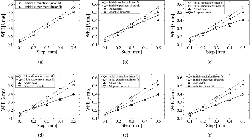
The absolute positions of the lenses within the barrel, which were moved in the process of repeatedly attaching and detaching the IO module after the initial experiment, could not be measured, and thus the relative distances among the lenses were different. Accordingly, additional compensation experiment was performed in the status where the distances among the interferometer, IO module, and spherical mirror changed slightly. As for the compensation equation for increasing the prediction accuracy of the resulting values, a straight line was drawn using a fitting line equation (Fig. 6a), and based on this graph, experiment was performed using a total of five steps for the Z-axis (despace), which had a large effect on the change of WFE as shown in Fig. 5, by adding 0.2 mm and 0.4 mm steps to the existing three steps.

Fig. 6 is a graph that shows the process of obtaining an adaptive fitting line. Fig. 6a shows the fitting lines of the simulated values, which were calculated from the initial values, and the experimental values. From Fig. 6b to Fig. 6f, added data was applied to the simulation fitting line one by one, and the resultant fitting line was obtained by recalculation. The dark triangles represent the added points. Fig. 6 shows the case of the RT-NV condition. For the RT-V and LT-V conditions, the same process was applied.

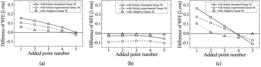
Based on the resultant values of the wavefront error measurement, Fig. 7 shows the differences among the fitting line of the simulated linear fit, the fitting line of the experimental linear fit, and the adaptive fitting line. Fig. 7a shows the differences at the RT-NV condition, Fig. 7b shows the differences at the RT-V condition, and Fig. 7c shows the differences at the LT-V condition.

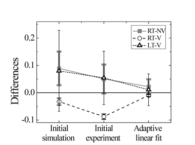
In the case of the difference between the simulated and the resultant values of the initial experiment, for the RT-NV condition, it gradually decreased; for the RT-V condition, it decreased and also increased although the variation was small; and for the LT-V condition, it gradually decreased but there seems to be a possibility to increase considering the shape of the graph. On the other hand, the adaptive fitting line showed a gradually decreasing trend at all the conditions. Fig. 8 shows the trend of the overall differences in the values. For the error bar, the standard deviation was used, similar to Fig. 5. For the LT-V condition, the difference between the simulated and the experimental values was the smallest, compared to the other conditions, as shown in Fig. 8. It is thought that this is because the IO module of IGRINS was elaborately designed and manufactured so that the internal lenses could be aligned at LT-V condition. On the other hand, it is thought that for the RT-V and RT-NV conditions, the differences were large because the changes of the internal environment of the IO could not be examined and thus the errors became relatively large compared to the simulation.

When the differences were the smallest by adding five added points to each condition, the fitting line equations were y=0.613x+0.090 for the RT-NV condition, y=0.944x+0.112 for the RT-V condition, and y=1.134x+0.001 for the LT-V condition. Based on these equations, the prediction accuracy of the initial simulation was calculated to be 0.067±0.030 λ rms WFE, the difference between the initial experimental values and the initial simulation was calculated to be 0.064±0.021 λ rms WFE, the prediction accuracy of the developed compensation fitting line was calculated to be 0.014±0.007 λ rms WFE, and especially for the LT-V condition, it was 0.011±0.058 λ rms WFE.

The purpose of the ‘no adjustment’ design philosophy is to minimize time and cost by minimizing assemblyalignment processes through the precise manufacture of opto-mechanical parts. Accordingly, the barrel used in this study was manufactured by precise mechanical machining, and as shown by the results of this study, the wavefront error could be precisely predicted with a prediction accuracy of 1/100 λ rms. Therefore, the precise manufacture of opto-mechanical parts would enable more precise prediction of optical performance depending on temperature and pressure environments, and inversely, precise optical performance prediction techniques would assist manufacture opto-mechanical parts more precisely. In this study, an optical performance prediction technique was developed using a compensation fitting line so that experimental values could be more precisely predicted at each condition. With the developed technique, optical performance can be predicted in advance as it changes among RT-NV, RT-V, and LT-V conditions. Therefore, it is expected that final performance could be quickly achieved by performing assembly and alignment while minimizing the change of condition.