The modulation transfer function (MTF) is a widely used indicator in assessments of remote-sensing image quality. This MTF method is also used to restore information to a standard value to compensate for image degradation caused by atmospheric or satellite jitter effects. In this study, we evaluated MTF values as an image quality indicator for the Geostationary Ocean Color Imager (GOCI). GOCI was launched in 2010 to monitor the ocean and coastal areas of the Korean peninsula. We evaluated in-orbit MTF value based on the GOCI image having a 500-m spatial resolution in the first time. The pulse method was selected to estimate a point spread function (PSF) with an optimal natural target such as a Seamangeum Seawall. Finally, image restoration was performed with a Wiener filter (WF) to calculate the PSF value required for the optimal regularization parameter. After application of the WF to the target image, MTF value is improved 35.06%, and the compensated image shows more sharpness comparing with the original image.
The world’s first geostationary ocean remote-sensing instrument, the Geostationary Ocean Color Imager (GOCI), was launched on 27 June 2010 to monitor the marine environment of the Korean peninsula. GOCI provides eight image acquisitions a day for the Northeast Asian region and can be applied to various research areas, such as suspended sediment and chlorophyll concentration monitoring, in addition to providing timely warning of marine dangers. GOCI images have a 500-m spatial resolution, consisting of 16 slot images for a 2500 × 2500 km area, centered at 130°E, 36°N (Table 1) (Ryu et al. 2012). Calibration and image quality control and enhancement are crucial to the successful operation of the GOCI system. The precise image quality assessment for increasing the applicability and scientific data accuracy uses a modulation transfer function (MTF) and signal-to-noise ratio (SNR) comparison.
[Table 1.] General specifications of the Geostationary Ocean Color Imager (GOCI).
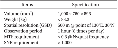
General specifications of the Geostationary Ocean Color Imager (GOCI).
In image-based MTF measurement methods, the knifeedge method, point source method, and pulse method are widely used to determine whether the targeted optical system performance has been achieved in real instrument operation. These methods also account for factors influencing the space environment which can change the resulting image quality (Helstrom 1967, Holst 2008, Hwang et al. 2008, Viallefont 2010, Yin et al. 1990). A common concept among the three methods is the characterization of the spatial quality of the remote-sensing systems with the Fourier transform of the point spread function (PSF) of the target image. First, the knife-edge method uses an edge spread function (ESF) created by a well-contrasted edge area in the target image. The line spread function (LSF) is then computed by a simple discrete differentiation of the ESF; the MTF value is obtained by the Fourier transform of the LSF in the last step (Choi 2002, Viallefont 2010, Viallefont & Leger 2010). The other two methods, the point source and pulse methods, are similar to the knife-edge method, but these methods obtain the PSF values directly from a particular point source and pulse. In this case, the MTF value is computed by Fourier transformation of the PSF (Choi 2002, Leger et al. 1994).
In this study, we focused on the proper MTF estimation method using the natural target and GOCI image enhancement with MTF compensation. If we assume that the remote-sensing PSF blurs the acquired image caused by atmospheric effects, satellite conditions, and other space environment effect, then MTF compensation methods are usually used to correct image degradation with estimating blurred PSF. These MTF compensation methods include the use of an inverse filter (IF), a pseudo-inverse filter (PIF), and a Wiener filter (WF) (Demoment 1989, Jeon et al. 2012). Despite the aforementioned techniques developed and used for various remote-sensing image investigations (Reichenbach et al. 1995, Rojas et al. 2002, Ruiz & Lopez 2002, Wu & Schowengerdt 1993), image enhancement for GOCI has never been studied with MTF compensation using the Wiener Filter.
This paper begins with a description of the GOCI system, MTF estimation, and compensation technique in Section 1. The methodology used to estimate MTF with the pulse method and image enhancement by Wiener filtering as compensation is described in Section 2. Section 3 presents the enhanced image results with MTF compensation for the Saemangeum area. Conclusions are presented in Section 4.
2.1 Image-based MTF assessment method: pulse method
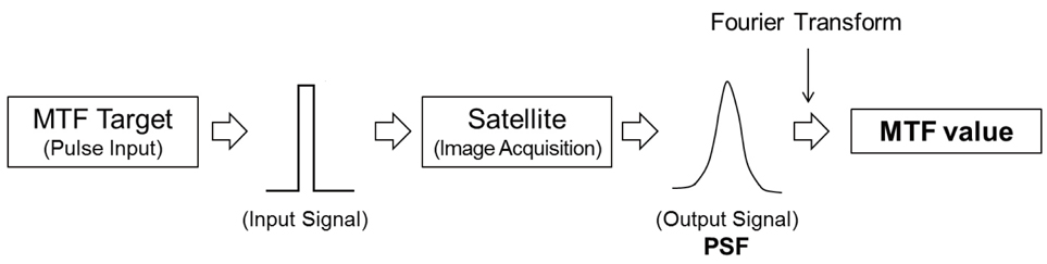
Fig. 1 shows the general process of MTF assessment, using the pulse method. First, a PSF value is obtained from the pulse target in an acquired image. The image is then Fourier transformed from a PSF to an MTF value (Helstrom 1967). The target area for the pulse input signal should be smaller than the spatial resolution of the remote sensor. The MTF result is more accurate when the Nyquist frequency is less than the first zero-crossing frequency in the Fourier transform step (Tzannes & Mooney 1995). Fig. 1 shows the blurring of an image of a rectangular-shaped input pulse, due to environmental effects, resulting in a PSF value that has a curve-shaped output. The pulse shape is determined by the size of the target pulse width. However, because noise is included in the pulse signal, a PSF curve-fitting model should be applied, such as the Gaussian function, polynomial curve, or Fermi function, which are commonly used for this purpose (Choi 2002, Jo et al. 2008, Smith 2006). For this study, we used a Gaussian function to fit the PSF curve, defined by

where where σ and μ are the standard deviation and median value of the Gaussian curve, respectively. These two parameters will be used in the principle values of the WF.
2.2 Remote-sensing image compensation method: Wiener filter (WF) method
The purpose of image restoration is to remove noise from remote-sensing images and to approximate the original image via estimation with an ideal degradation model.
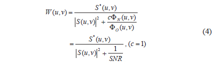
Among image restoration methods such as IF, PIF, and WF, we selected the WF method which minimizes the error in estimating the ideal image from the noisy image by linear filtering (Demoment 1989). The computational process for the WF method used in this paper is given in Eqs. (2-4):


In Eq. (2), g(

We estimated the PSF of the target image using the WF method designed by Helstrom (1967). The WF value is denoted as
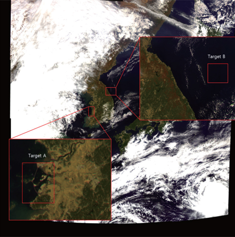
Fig. 2 shows the regions of interest for MTF and PSF value computation (Target A) and image-based SNR (Target B). The Target A area corresponds to the Saemangeum seawall on the west coast. The MTF in this case (i.e., the complex coastline) was estimated using the pulse method. A constant signal from the East Coast area (Target B) was selected to estimate the SNR of the image and will be used as the major element of the WF. The detailed locations and sizes of the two target areas are listed in Table 2.
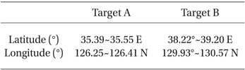
Target image areas for the modulation transfer function (MTF) and signal-to-noise (SNR) estimation.
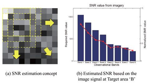
The Saemangeum seawall has an average width of 290m, which was used to estimate the MTF value. The width of the image was estimated to be 312.02 m with a geometric slope of 67.16˚. The targe width as a pulse in the input signal fits the criterion of being smaller than the spatial resolution of a pixel (500 m) and is thus appropriate for our analysis. To obtain an image-based SNR, we selected an area in Target B with a chlorophyll value of less than 0.07 mg m-3. This SNR is based only on the image noise and excludes fluctuations that may exist due to ocean conditions (Hu et al. 2012).
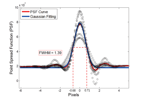
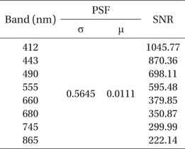
To obtain the PSF and SNR values for the WF, the pulse signal for the target area was converted to a distribution function for each row. In Fig. 3, the radiance value for PSF for each row was ordered by the peak point at 0 pixel position (marked by ‘black circular sign’). Then, the average values for the fitted curve were used to construct the PSF curve (‘Red line’ in Fig. 3). A Gaussian fitting curve was used to match the PSF curve as a normal distribution (‘Blue line’ in Fig. 3); from this, we computed where σ and μ are the standard deviation and median value of the Gaussian curve, respectively. These two parameters will be used in the principle values of the WF. and μ, which were 0.5645 and 0.0111, respectively. Additionally, the estimated full width at half maximum (FWHM) of the fitted PSF curve was 1.3886 and did not exceed two pixels.


The SNR values used in the WF for the target area (Target B) were calculated using Eq. (5) (Fig. 4). To achieve the SNR from the nearly homogeneous area in the imagery, a small square (n × n) window of pixels (in this paper, 5 × 5 pixels) was moved within the target area (100 × 100 pixels for GOCI) by one-pixel steps to obtain the average value of where σimage (counts) and the standard deviation value of where σnoise (counts), as shown in Fig. 4b.
[Table 3.] Control parameter for the MTF compensation with WF method.
Control parameter for the MTF compensation with WF method.
Table 3 summarized the image restoration parameter of PSF and SNR that we calculated where σ and μ are the standard deviation and median value of the Gaussian fitting curve at the Target area ‘A’, and SNR values are estimated from each band image signal of the Target area ‘B’. With those parameters, we applied WF to compensate the image, and discussed the results in the Section 3.3.
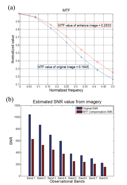
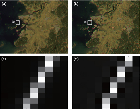
In Fig. 5a and b, two red-green-blue (RGB) composite image (R: 680 nm, G: 555 nm, B: 412 nm) obtained at UTC 03 on 16 October 2012 are compared that the MTF compensated image illustrates the improved image quality in aspect of sharpness and contrast in the coastal area near the Saemangeum seawall and inland river boundary. We compared the MTF results between the original and enhanced images after estimating the PSF with the WF method to confirm this difference quantitatively with using the target areas as shown in Fig. 5c and d.
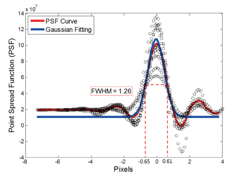
The FWHM and PSF values of the reconstructed image using the WF were improved significantly compared with the original image. In Fig. 6, the FWHM and the where σ value of the standard deviation of the Gaussian function improved from 1.3886 to 1.2600 and from 0.5645 to 0.4924, respectively. Finally, the MTF value at the Nyquist frequency increased by 35.06% (0.2533) compared with the source image as shown in Fig. 7a. On the other hand, SNR values estimated in the Target ‘B’ are decreased for all bands. In case of band-8, the estimated SNR value based on the image is changed from 222.14 to 155.62.
This study was performed to evaluate the image quality of the GOCI system with the first suggested technique using the natural target, as well as to improve its quality with MTF compensation based on the WF method. We measured the MTF for a natural target, the Saemangeum seawall, at UTC 03 on 16 October 2012 and designed a WF with a PSF value, on the basis of MTF processing and SNR values obtained for seawater. After application of the WF to the target image, the enhanced image was generated with a 35.06% improved MTF value compared with the original image.
Despite the 500-m spatial resolution of the GOCI satellite image, it is difficult to estimate the exact PSF value. In addition, the SNR values are also relatively estimated based on the image, and that is reason why the SNR value is underestimated comparison with requirement. Although SNR value is decreased from applying MTF compensation, the enhanced image having high MTF value can be practically used in monitoring works and researches in coastal area. Furthermore, the relationship between ocean color product accuracy and MTF enhanced image will be discussed with further investigation in the near future.
Thus, the significance of this paper lies in the improvement of the image quality using the wellconstructed WF method with Gaussian curve fitting. With the restoration results, the complexities of the west coast area and its islands were clearly distinguished with the naked eye as a result of the improved image quality. Additionally, this work is firstly suggested to estimate in-orbit MTF and SNR value, and generate the MTF compensated image of geostationary orbit satellite for ocean monitoring. We believe that the results of this study are expected to provide a more accurate description of the coastal regions for improvement in image processing such as cloud detection for atmospheric correction and ocean color data in coastal area.