Due to the continuous space development by mankind, the number of space objects including space debris in orbits around the Earth has increased, and accordingly, difficulties of space development and activities are expected in the near future. In this study, among the stages for space debris removal, the implementation of a vision-based approach technique for approaching space debris from a far-range rendezvous state to a proximity state, and the ground test performance results were described. For the vision-based object tracking, the CAM-shift algorithm with high speed and strong performance, and the Kalman filter were combined and utilized. For measuring the distance to a tracking object, a stereo camera was used. For the construction of a low-cost space environment simulation test bed, a sun simulator was used, and in the case of the platform for approaching, a two-dimensional mobile robot was used. The tracking status was examined while changing the position of the sun simulator, and the results indicated that the CAM-shift showed a tracking rate of about 87% and the relative distance could be measured down to 0.9 m. In addition, considerations for future space environment simulation tests were proposed.
With the continuous space development, the activities of satellites have become essential part of mankind. For a long time, satellites have performed a lot of activities in various fields (e.g., weather forecast, long-range communication, Earth environment and seawater observation, military missions, and space exploration). In the future, they are expected to perform more diverse tasks such as the fueling, repair, and mission change of satellites with the use of servicing satellites. However, the disposal of satellites which completed their missions has not been properly considered so far, and other uncontrollable satellites or part of space launch vehicles revolving around the Earth have collided with space objects and have produced a lot of space debris. Especially, the amount of space debris has abruptly increased due to the interception experiment of Feng-Yun 1C from China in 2007 and the collision between IRIDIUM 33 from the United States and COSMOS 2251 from Russia in 2009. Currently, the number of space debris for entire orbits is estimated to be about 1012 for those with a diameter of more than 0.1 mm, and about 750,000 for those with a diameter of more than 1 cm. Among these, the number of cataloged space objects is estimated to be about 17,000 (Krag 2013). The collision between space debris and satellites operated by various countries causes the breakdown of the satellites, and significantly affects the missions. To prevent this, many efforts have been made to avoid collision in advance via continuous monitoring, but it cannot be an ultimate solution.
On the other hand, to prevent the formation of space debris, countries operating satellites have recently proposed the ‘post-mission disposal (PMD)’ regulation, by which launched satellites should be decayed within 25 years of the mission completion, and are actually designing missions that follow the regulation. NASA reported that if the ‘active debris removal (ADR)’, by which 5 pieces of space debris are removed every year, is simultaneously performed along with PMD, the low Earth orbit environment could be stabilized by maintaining the current number of space debris (Fig. 1) (Liou 2009), and also reported that if more than 5 pieces of major space debris are removed every year for 200 years from 2020, the increasing trend could become more gentle (NASA ODPO 2007).
Based on the above results, various methods for removing major space debris have been studied in many countries around the world. The methods that have been studied include a method which induces de-orbiting by attaching a tether, which has been conducted by the electromagnetic force around the Earth, to space debris (Nishida et al. 2009), a method which induces the de-orbiting of space debris using an ion-beam and a laser from the Earth’s surface or on the orbit (Merino et al. 2011, Phipps et al. 2012), a method which induces de-orbiting by deploying a sail loaded on a satellite and by receiving the solar wind (Stohlman & Lappas 2013), and a method which uses a capture system that removes a single or multiple pieces of small space debris using a robot-arm or nets (Benvenuto & Carta 2013, Richard et al. 2013).
Also, overseas research institutes have constructed various ground-based test beds for testing the space orbit techniques (e.g., rendezvous, docking, and proximity operation) that are applied to space debris removal and service satellite activities. Especially, vision-based ground test beds focused on simulating satellite motion and space environment. For the simulation of three-dimensional motion, a configuration using a 6-DOF robot (Wimmer & Boge 2011) and an underwater test bed configuration (Atkins et al. 2002) have been constructed. For the simulation of two-dimensional motion, a configuration, in which a floor was made to have a frictionless state for floating condition, has also been constructed (Romano et al. 2007). In Astrium, INRIA/IRISA, a ground-based test has been performed, which acquires distance information using the contour motion of a space object as the image information, without a marker or prior information (Petit et al. 2011). In Korea, research on a space debris removal system is also in progress along with the development of a space debris collision risk management system (Kim et al. 2013).
In this study, the implementation of an algorithm for a vision-based approach technique, and the ground test results of an approach (rendezvous) platform using a lowcost test bed were described as the preliminary research on the development of a capture system for active debris removal.
2.1 Vision sensor for space environment
Core space technologies such as rendezvous and docking require precise technology, and thus have been carried out in manned condition. However, as manned space missions incur a lot of cost and have a high risk level, studies on unmanned missions have been actively performed to replace manned missions. Accordingly, for a more accurate decision in proximity condition, it is necessary to select a sensor that is appropriate for the condition. Also, a method, which sends the data obtained from the sensor to the ground, processes the received data on the ground, and again transmits the processed data to the spacecraft, leads to a time delay, and thus is not appropriate for prompt missions. In this case, an on-board system needs to be constructed, which can process the sensor input data in real time at the platform. Fig. 2 shows the navigation sensors that are needed to perform rendezvous and docking on a space orbit, depending on the distance. For about 100 km which is the beginning stage of the rendezvous, a global positioning system (GPS) is used to initiate the far-range rendezvous. For the mid- and close-range rendezvous, radar and a vision-type sensor are appropriate, and for the proximity condition of less than 5 m, a laser range finder is used.
For the ground test range of this study, the approach is assumed to have been completed, using GPS data information, down to about 100 m that is the range in which a vision-type sensor can be used. Then, starting from this position, it is assumed that the approach to a space object is carried out down to just before the proximity operation such as docking and berthing. For the vision-type sensor, a stereo camera was used so that the distance to an object without prior information on the size and shape could be measured.
2.2.1 Vision algorithm for the tracking of space debris
Object tracking using images has been applied to various situations such as face tracking and surveillance (Hsia et al. 2009) and object chasing and sports game analysis (Kim et al. 2010), and the algorithms that have been generally used include difference image, optical flow (Choi et al. 2011), SIFT, SURF, contour tracing, mean-shift, and CAM-shift (Salhi & Jammoussi 2012).
The difference image extracts a foreground by subtracting an image including the foreground from a background image, and is typically appropriate for surveillance at a fixed position. The optical flow is a method in which feature points within an image estimate the motion between frames, and can be used when a background and an object move together. The mean-shift tracks an object by searching local extrema from the density distribution of data. For the CAM-shift, size modification is enabled regarding the tracking window of the mean-shift.
Space environment has a simpler background compared to ground environment, but the background change within an image is very abrupt because the motion of a camera and a platform is faster than those on the ground. For the difference image and optical flow, object recognition is relatively not easy because the change of background motion is similar to that of tracking object motion. For the mean-shift and CAM-shift that use the density distribution of data, object recognition in space environment is relatively easy because the environment is simple. Also, for object tracking in space environment, the object size at the beginning of rendezvous is significantly different from the object size just before docking, and space debris exists in a tumbling state that is uncontrollable and unstable because of collision. Therefore, the CAM-shift, which is capable of tracking window modification, is appropriate for space debris tracking.
The CAM-shift is based on the mean-shift, and operates by continuously updating the size of the tracking window. The mean-shift algorithm tracks a specific object by searching part of the tracking area, and the necessary information such as the position of the center of gravity, the width and height of the tracking window, and the coordinate information are calculated using the 0th, 1st, and 2nd moment (


The coordinates of the center of gravity for the tracking window (

The direction angle between the principal axis of the image and the tracking window (


Fig. 3 is a flowchart that shows the process by which the image information inputted from the camera is calculated at the vision system using the CAM-shift and the Kalman filter.
2.2.3 Range measurement using disparity
In space environment, a distance change is obtained by measuring the time for the transmission and reception of electromagnetic signals or by integrating velocity all over the time. In the case of a method using images, a distance can be measured using the proportion of an object in the vision image with prior information on the object. Another method is to use the stereo vision that extracts depth information using more than two images. The stereo vision acquires images in a form similar to the visual structure of a human, and generates a depth map by calculating the displacement of the feature points of the left and right images using triangulation. Fig. 4 shows the geometric configuration of the stereo vision. The
The point P of the real world appears as

Using the coordinates and parameters of the image plane, the coordinates of the real world,


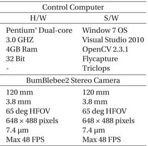
Fig. 5 shows the configuration of the test bed system for active debris removal. For the mobile robot, NTCommander- 1 (Ntrex Co., Ltd.) was used. For the vision sensor, Bumblebee 2 Stereo Camera (PointGrey, Inc.) was used, and the specifications of the vision sensor and the control computer are summarized in Table 1. As for the mobile robot, a two-wheel type mobile robot, which has similar motion to the satellite motion where a satellite moves forward by setting a direction using an attitude control system, was used. For the vision algorithm, the OpenCV library was used, and for the distance measurement algorithm, the Flycapture and Triclops, which are the libraries of Bumblebee 2 Stereo Camera, were used. The test was performed at a stereo camera frame rate of 30 FPS and an image size of 640 × 480 pixels.
[Table 1.] Chaser system speculation.

Chaser system speculation.
The tracking target object was a model of Chollian Satellite (Communication, Ocean and Meteorological Satellite) shown in Fig. 6. The Chollian Satellite model used in the test had a size of 11 cm × 8 cm × 18.5 cm (width × length × height), which was a 1/50 scale model of the actual satellite.
Fig. 7 shows the position of the sun simulator during the test. The differences in the sunlight directions were compared by changing the included angle between the field of view of the camera and the sun simulator. As summarized in Table 2, P1 is the forward direction of the mobile robot; P3 is the side of the tracking target; P2 is between P1 and P3; and P4 is above the tracking target. Table 2 shows the straightline distance between the light source of the sun simulator and the target satellite model, and the distances in each direction.
[Table 2.] Position of sun simulator.
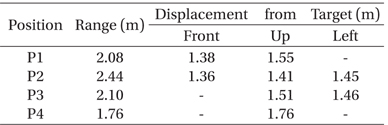
Position of sun simulator.
Fig. 8 shows the implemented test bed. To remove the effect of the reflection from the sun simulator, black paper was attached to the periphery. The tracking target object was assumed to be incapable of attitude control, and thus it was hung on a string and rotated randomly.
The test was performed 3 times at each sun simulator position (P1 ~ P4), for a total of 12 times. For example, the second test at position P1 was expressed as P1-2. Fig. 9 shows the image capture data of the P3-2 test, and it approaches the target in the order of (a) to (f ). From a relative distance of 3 m, the test was performed while continuously measuring the distance using the vision algorithm. (a) represents the 2.04 m distance, (b) represents the 1.77 m distance, and (c) represents the 0.95 m distance. For (d) ~ (f ), the distances could not be measured.
Fig. 10 shows the histogram of the target satellite model at positions P1 ~ P4. As the color of the light from the sun simulator was vermilion and the color of the satellite model was yellow, the color appeared reddish. For P1 and P3, yellow color was also observed because much light, which had been reflected from one side of the satellite, was received. Especially, for P1, it was the brightest because the amount of the reflected light, which had been received by the camera, was the largest. For P4, yellow color was not observed and it appeared red because relatively weak light was incident on the front and the side that the camera faced. For P2, yellow color was also not observed and it also appeared red because the distance was relatively far.
Table 3 shows the tracking rate of the CAM-shift tracking algorithm for each case. The maximum tracking rate was more than 97% at P1-2, and the minimum tracking rate was about 74% at P4-1. The results depending on the sun simulator position indicated that P3 showed the highest tracking rate. For P4, it is thought that the amount of received reflection was small because the light was incident only on the upper part of the target satellite model. For P1 and P2, it is thought that the tracking rate slightly decreased because white noise occurred as the light was incident on the same direction as the moving direction. For P3, it is thought that the tracking was satisfactory because the light could be stably incident on the target satellite model. For the entire test, the average tracking rate was about 87%.
[Table 3.] Chaser system speculation.

Chaser system speculation.
The graph in Fig. 11 shows the tracking pixel error of the Kalman filter, which has been used to improve the tracking performance of the CAM-shift algorithm. In the early stage of the tracking, an error occurred to some extent because the pixels of the tracking window changed abruptly to search the object after the tracking window setting of the CAM-shift algorithm, but during the object tracking, the error was less than 10 pixels, indicating that the tracking was satisfactory. However, the results in the latter stage object tracking and in Fig. 11b indicated that a large error, which was more than 20 pixels in the early stage, was observed. As shown in Table 3, the tracking rate was low at P2-2. Therefore, it is thought that the error became large in order to search the accurate center of the tracking window. Also, it is thought that when the distance to the object was less than 50 cm, the center of the tracking window changed abruptly and could not converge since the target satellite model occupied large area of the image as shown in Fig. 9f.
The graph in Fig. 12 shows the results of the distance measurement depending on the sun simulator position. As the disparity values were not calculated at some frames, there were intervals with a constant distance. However, for most of the tests, the tracking started at a relative distance of 3 m, and the distance was measured down to about 0.9 m. For all the case of P2 (Fig. 12b) and P4-3 (Fig. 12d), there were intervals with increasing distance, and it is thought that this was an error occurred during the direction change. For frame 288 of P3-2, a distance of 1 m was calculated, and it is thought that this value was calculated based on an outlier of the disparity at a proximity state to the target satellite model.
In Fig. 13, the trajectory was drawn using the position coordinate of the target satellite model (the P coordinate in Fig. 5) with the use of Bumblebee 2 Stereo Camera. This coordinate represents the relative coordinate of the target satellite model and the camera. If the X coordinate is 0, it indicates that the mobile platform is aligned with the target satellite model. As shown in Eq. (16), the X coordinate was calculated based on the straight-line distance Z. Therefore, the trajectory was drawn excluding the values where the distance Z was less than 0.9 m. For the coordinates with a relative distance of down to 0.9 m, the X coordinate was mostly within 0.1 m, indicating that the mobile platform and the target satellite model were almost aligned. Therefore, it is thought that a normal close-range rendezvous state for proximity operation was successfully achieved.
In this study, a vision-based approach algorithm for active debris removal was developed, and the implemented algorithm was tested by constructing a ground-based space environment simulation test bed. For the continuous object tracking using only a vision sensor without the addition of other sensors, a stereo camera that can measure distances using a depth map was used. For the implemented algorithm, the CAM-shift, which is less affected by external environment and has high speed, was used, and the Kalman filter was added to improve the accuracy of the algorithm. For the mobile platform, a two-wheel type platform, which performs rotational and translational motion in the rotation direction of the motor and which can effectively simulate the motion of a satellite, was used. In the ground simulation test using the test bed, it was investigated whether the image tracking could be successfully performed in space, where the light environment condition is different from the ground. Especially, to examine the mission performance ability depending on the position change of the Sun while revolving around the Earth, the test was carried out by changing the incidence angle of the light. The test was conducted using the target satellite model at a distance of 3 m, and the CAMshift algorithm mostly showed a tracking rate of more than 70%. It is thought that the results were affected by the intensity of the light rather than the position of the sun simulator. The distance could be measured down to 0.9 m.
In the future, to implement a test bed for the study of a space debris removal system, the simulation of motion in space environment and the equivalence depending on the distance to a tracking object need to be considered, and especially, the effects of direct sunlight and Earth’s albedo need to be considered. As the stereo cameras used in this study were parallel, the distance measurement was difficult in the proximity state within a certain distance to the tracking object. Therefore, it is thought that the included angle between the two cameras needs to be changed or other type of sensors such as a laser range finder that is useful for proximity distance measurement need to be added besides the vision sensor.