The Sun is a variable star with periods ranging from minutes to years. In particular, the variability in its magnetic field strength affects the interplanetary space and in turn the Earth’s electromagnetical environment (Kane 1986, Prestes et al. 2006). To identify actual mechanisms and processes for the observed variation in geomagnetic activity, the 11- year solar cycle and associated variabilities have been actively studied in the last decades. From harmonic analysis of variations of key parameters in geomagnetic activity, such as, the proton number density and bulk speed of solar wind, the interplanetary magnetic field strength, the disturbance storm time index (Dst index), the Auroral Electrojet index (AE index), periodicities of ~ 11 years, ~ 5.3 years, ~ 3.5 years, ~ 1.9 years are found being meaningful (Kane 1997, Clúa de Gonzalez et al. 2001, Kane 2005, De Artigas et al. 2006). Those periodicities obviously correspond to the main solar cycle and its overtones. In addition, the annual variation in the weak-to-moderate categories of storm intensity has been found in the Earth’s neighborhood, which is due to the Earth’s orbital revolution. The annual geomagnetic activity distribution is characterized with maxima around the equinoxes and minima near the solstices. The cause of this seasonal variation is still a matter of debate but may be attributed to one or more of the three models known respectively as the equinoctial hypothesis, the axial hypothesis and Russell-McPherron mechanisms (Russell & McPherron 1973, Clúa de Gonzalez et al. 1993). Further studies show, besides, that the annual distribution of magnetically-disturbed days is more complex when events with high levels of storm intensity are considered. That is, the presence of an anomalous peak in July for the monthly number of days with value of Ap > 200 nT or Dst< -180 nT is reported (Clúa de Gonzalez et al. 2002). This occurrence seems to be common along the 12 solar cycles covered by these indices.

In these parameters mentioned above, the solar rotational periodicity of ~ 27 days and its subharmonics with shorter periods have been revealed (Mursula & Zieger 1996, Prabhakaran Nayar et al. 2001, Mendoza et al. 2006, Charan Dwivedi et al. 2009, Emery et al. 2011). The power spectra of Galactic cosmic ray (GCR) intensity during solar cycle 23 have also been analyzed (Singh et al. 2012). They have too shown the existence of a variety of prominent short- and mid-term periodicities of ~ 27 days, ~ 14 days, and ~ 9 days as well as annual, semi-annual and tri-annual variations of ~ 200 days. Furthermore, studies have discovered a strong 1.3-year variation in solar wind speed and geomagnetic activities, which is expected to be due to the evolution of coronal holes (Richardson et al. 1994, Mursula & Zieger 2000, Obridko & Shelting 2007, Ruzmaikin et al. 2008, Cho et al. 2014). Several studies are devoted to oscillations with a period of 1.3 years revealed at the bottom of the solar convection zone. Komm et al. (2003) and Howe et al. (2000) have found out that the 1.3-year periodicity at the base of the convection zone is most pronounced in the solar rotation rate at the equator of the tachocline. In recent years, nonetheless, the oscillation periods of 1.3 years in helioseismic measurements have not been as clear as earlier (Komm et al. 2006).

The aim of this study is twofold. Firstly, following variations of the power over the time, we associate modes with periodicities of ~ a month seen in signals observed in the interplanetary space and in the Earth’s magnetosphere. If the power of two different signals shows uncoupled temporal behaviors over the time, even though they show a significant peak at the same frequency in the power spectrum, they can be possibly argued that they are causally unrelated. Thus, it is insufficient searching for reported periodicities in order to causally correlate geomagnetic activity parameters, rather requires examining the temporal features of the power. In this present study, we focus on short periodicities of a factor of a month close to the solar rotational period. We are to attempt to obtain information on the temporal behavior of the power in an oscillatory signal by employing the time/frequency analysis. The time/ frequency analysis, for instance, the wavelet transform, is able to give variations of power or frequency of a mode with time. This analyzing technique is used in many fields of physics and engineering, such as, acoustics, geophysics, helioseismology, image processing (Park & Chang 2013). Secondly, we attempt to search for any signatures of influence on the space environment near the Earth by inner planets revolving around the Sun (see, Kim & Chang 2014). Supposed that the inner planets make its shadow up to the Earth’s orbit at 1 AU from the Sun and disturb the Earth’s space environment, there must be a periodic perturbative signal in geomagnetic activity data corresponding to the synodic period of inner planets. We thus attempt to find out a possible evidence of such a shadow by looking for consistent signals in the power spectra that can be ascribed to the passage of the shadow.

This paper is organized as follows. We begin with brief descriptions of data analyzed for the present paper in Section 2. We present and discuss results of Lomb-Scargle analysis of geomagnetic activity indices in Section 3. Results of the time/frequency analysis are subsequently presented and discussed in Section 4. We discuss a possibility of shadowing of inner planets to the Earth’s space environment in Section 5. Finally, we summarize in Section 6.

For the present analysis, firstly, we have used the mean daily velocity of the solar wind during the period from 1999 to 2012, which is obtained by the Solar Wind Electron, Proton, and Alpha Monitor (SWEPAM) on the Advanced Composition Explorer (ACE) spacecraft. We have also used the number density of protons (n_p in # cm^-3) in the solar wind during the same period. The proton density is observed by the same instrument on the ACE spacecraft. We have taken both data sets from the ACE Science Center website¹. Secondly, we have used the interplanetary magnetic field data observed during the same period by the Magnetic Field Experiment (MAG) on the ACE spacecraft. We adopt field values in the Geocentric Solar Magnetospheric (GSM) coordinate system, where the X-axis is parallel to the Earth-Sun line and Z-axis is the projection of dipole axis on the YZ plane of the Geocentric Solar Ecliptic (GSE) coordinate system, the Z-axis of the GSE coordinate system being the ecliptic north pole. Data have been taken from the ACE Science Center website1. Finally, we have used the Dst index and the AE index observed during the period from 1999 to 2012, in examining properties of the geomagnetic field. The Dst index is derived from a network of near-equatorial geomagnetic observatories that measures the intensity of the ring current. The Dst index is maintained at National Geophysical Data Center (NGDC)² and is available via FTP³. The AE index is, on the other hand, designed to provide a global, quantitative measure of auroral zone magnetic activity produced by enhanced Ionospheric currents flowing below and within the auroral oval. The AE index can also be downloaded via FTP⁴ of NGDC sites.

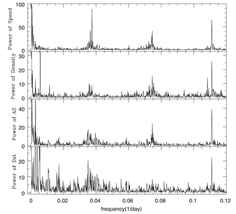
In Fig. 1, we show Lomb-Scargle periodograms of the velocity of the solar wind, the number density of protons in the solar wind, the AE index, the Dst index as a function of frequency in units of (), from top to bottom, respectively. Time series of data is taken during the period from 1999 to 2012. The power shown here is in an arbitrary unit. The periodogram analysis method developed by Lomb and Scargle is particularly appropriate for the analysis of unevenly sampled data (Cho & Chang 2011). This analysis method is basically same as Fourier analysis and sine curve fitting analysis. One of main advantages of this method is that the significance of a peak in the periodogram can be easily estimated, with a so-called false alarm probability. In plots, most conspicuous peaks in common are at the frequency of ~ 0.037 , ~ 0.074 , ~ 0.111 , when ignoring peaks whose frequency is less than ~ 0.01 , which we will come back to discuss later on in Section 5. They are the fundamental mode and its overtones, corresponding to periodicities of ~ 27 days, ~ 13.5 days, ~ 9 days. We note as other reports point out that the fundamental frequency is due to the solar rotation period. One might note that there is a barely recognizable peak at ~ 0.017 which is a half of ~ 0.037 .

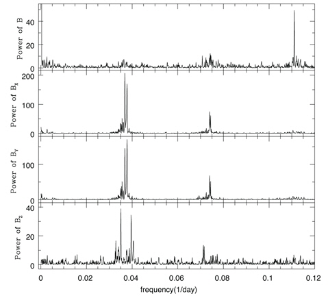
In Fig. 2, we show Lomb-Scargle periodograms of magnitudes in the interplanetary magnetic field, B and in its three components of the GSM coordinate system, B_X, B_Y, B_Z as a function of frequency in units of , from top to bottom, respectively. The power is in an arbitrary unit. Even though the main peak with the fundamental frequency due to the solar rotation and its overtones are clearly seen, their appearance is somewhat different each other. For example, in the power spectrum of B, the peak of the second overtone is largest. On the other hand, the peak of the second overtone can be hardly seen in the power spectra of B_X, B_Y, B_Z. As for the peaks of the fundamental mode and the first overtone, they are the other way around. It should be further mentioned another interesting point we note. The peaks in the power spectrum of B_Z appear to be split due to an unknown agent. Such a splitting can be seen in nature, or can be made by a frequency-modulation system, such as, a frequency-modulation (FM) radio (Chang 1995). In helioseismology, the rotational rate as a function of the solar radius is estimated by measuring such a rotational splitting of modes. And when a carrier wave is frequencymodulated by a square wave, the power spectrum of the carrier wave shows two distinctive peaks in the vicinity of the sidelobe. We suspect that the monthly variation in the southward component of B due to the solar rotation seems somehow modulated. As a record, the splitting is ~ 0.005 which corresponds to a time interval of ~ a half year. The third point to make is that on the contrary to Fig. 1, the power spectra is quite clean in the part where the frequency is less than ~ 0.02 . It could mean that the interplanetary magnetic field is less disturbed by a long-term variational process.

Compared to the Fourier transform, the Gabor transform GT is effectively a harmonic analysis with a running temporal window having a Gaussian shape, centered at a particular time t₀. The Gabor transform is thus defined as

where S(t) is the signal as a function of time t, G(t) is the window function, ν is the cyclic frequency. In the above form the wavelet transform WT can be considered as a transform of a signal derived from an original wavelet by dilation in time. That is, it is defined as

where d is a dilation coefficient. Naively speaking, the wavelet transform is the correlation of the signal S(t) and a running wavelet W(t). Then, a wavelet coefficient WT depends on two parameters: the time t₀ and the dilation coefficient d. Thus it will provide information around time t₀ and around frequency ν = 1/d. Its squared modulus is proportional to the power of the signal. This information is displayed in two-dimensional plots, showing variations of the energy with time and frequency. In other words, the temporal information is obtained by computing the correlation, which is a function of finite duration in time. The shape of the window is also an important parameter. It will allow optimization in time and in frequency of the information extracted. For the present analysis, we adopt the Morlet wavelet transform.

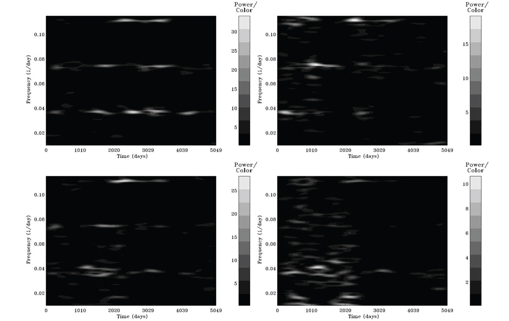
In Fig. 3, we show results from the wavelet transform analysis of the data. The horizontal axis represents time in day counting from the beginning of the data set, and the vertical axis the cyclic frequency in . The power is shown in gray scale, which is scaled by the mean value of the noise so that the signal-to-noise ratio can be assessed. In the top panels, results of the velocity of the solar wind and the number density of protons are shown from left to right. In the bottom panels, we show results of the AE index and the Dst index from left to right. As seen in Fig. 1, several high power peaks appear at ~ 0.037 , ~ 0.074 , ~ 0.111 , whose periods correspond to ~ 27 days, ~ 13.5 days, ~ 9 days, respectively. For the mode with the frequency of ~ 0.037 , temporal behaviors are akin, except the case of the proton density in the solar wind. That is, power of the proton density at this frequency appears to be very weak in time at about 1500, 3230, 4040 days, compared with results of others. In terms of the mode physics, this mode is likely to be excited by a somewhat different way. For the mode with the frequency of ~ 0.074 , while temporal behaviors of the solar wind velocity and the AE index are consistent, those of the proton density and the Dst index look different. Specially, this particular mode disappears in the case of the Dst index after 2000 days in time. On the other hand, for the mode with the frequency of ~ 0.111 , temporal behaviors of 4 parameters apparently coincide quite well.

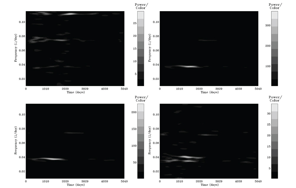
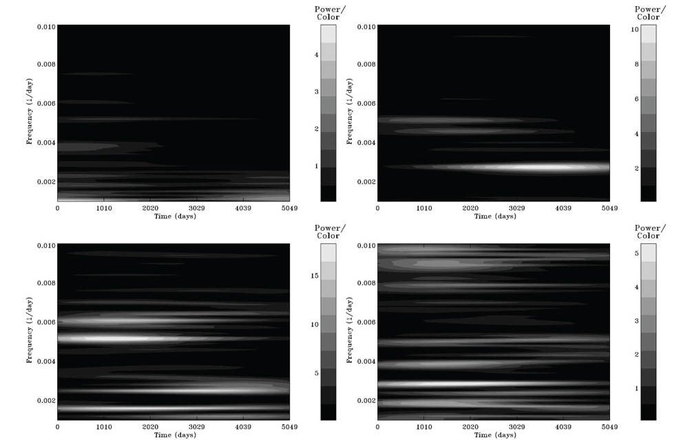
In Fig. 4, we show results from the wavelet transform analysis of the interplanetary magnetic field strength. The horizontal axis represents time in day counting from the beginning of the data set, and the vertical axis the cyclic frequency in . The power is shown in gray scale, which is scaled by the mean value of the noise. In the top panels, results of the mean magnetic field strength(B) and x-component of the interplanetary magnetic field in the GSM coordinate system are shown from left to right. In the bottom panels, we show results of y- and z-components of the interplanetary magnetic field from left to right. Generally speaking, plots agree to power spectra shown in Fig. 2 quite well. For instance, in the plot of left upper panel a strong peak at ~ 0.111 in the power spectrum of B is seen as can be found in Fig. 2. Peaks at ~ 0.037 and ~ 0.074 in the power spectra of B_X, B_Y and B_Z in Fig. 2 can be found in other panels. It is interesting to note, however, that all the powers seen in the power spectra are concentrated at ~ 1500 days in time and cannot be seen in the second half of the observing time.

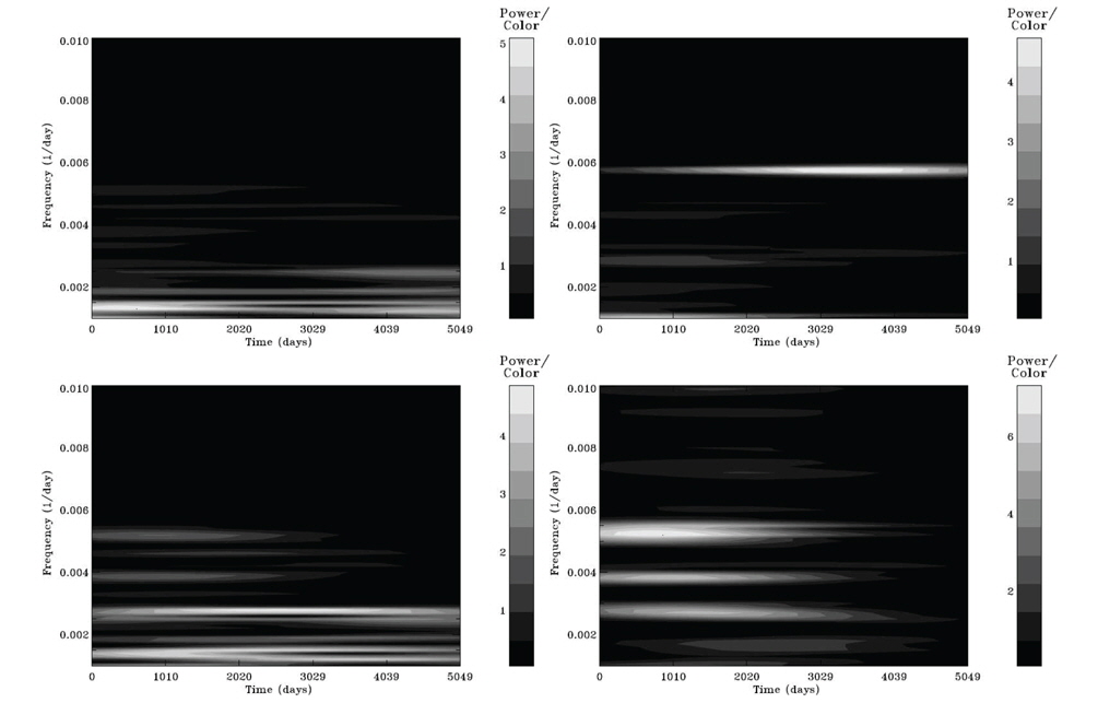
Here, we are particularly interested in the power spectrum of the frequency range where a recurrent perturbative signal in geomagnetic activity data due to the inner planets revolving around the Sun can be revealed. We zoom in the power spectrum to the frequency range including frequencies that correspond to the synodic and sidereal periods of inner planets, Mercury and Venus. By doing so, we attempt to search for any signatures of influence on the space environment near the Earth by inner planets revolving around the Sun.

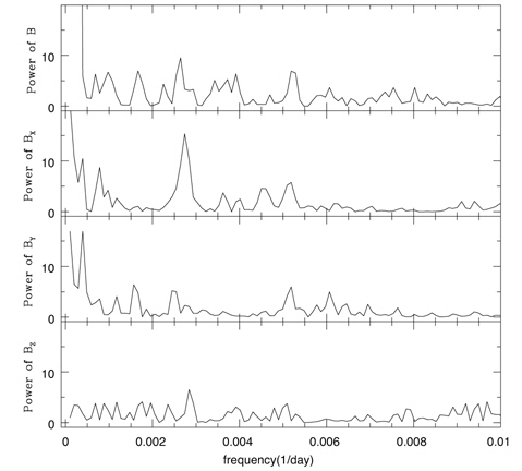
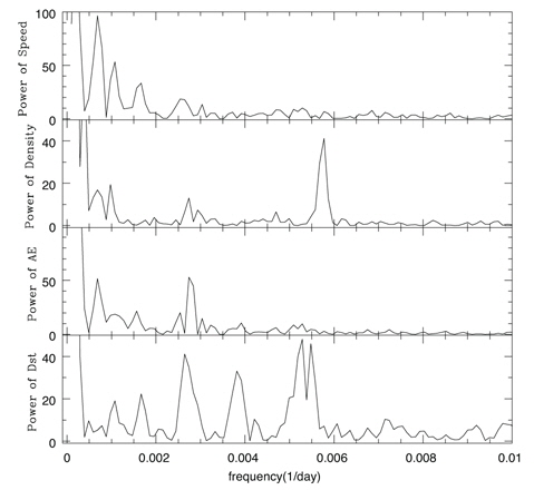
In Figs. 5 and 6, we show Lomb-Scargle periodograms of the velocity of the solar wind, the number density of protons in the solar wind, the AE index, the Dst index, and those of B, B_X, B_Y, and B_Z as a function of frequency in units of , respectively. The power is in an arbitrary unit. The frequencies corresponding to 1 year and a half year are ~ 0.0027 and ~ 0.0054 , respectively. Evident peaks can be found at those frequencies. Note, however, that only some of parameters show such a peak at those frequencies, which means that some parameters, such as, the solar wind velocity, are not annually modulated.

The sidereal periods of Mercury and Venus are 87.97 days and 224.70 days, respectively. The synodic periods of Mercury and Venus are 115.88 days and 583.92 days, respectively. Corresponding frequencies are ~ 0.0017 , ~ 0.0044 , ~ 0.0086 , ~ 0.0114 . Noticeable peaks do not emerge at those frequencies in power spectra shown in Figs. 5 and 6. There seems a vague hint that some peaks appear at ~ 0.0017 in the power spectra of the solar wind velocity, the Dst index, B, and B_Y . In order to see if they are positively compatible peaks, we show results from the wavelet transform analysis in Figs. 7 and 8 as we did in Figs. 3 and 4. Since modes at frequencies are not found except one at ~ 0.0017 , here we only consider the mode with the frequency of ~ 0.0017 which corresponds to the synodic period of Venus. Temporal behaviors of the mode in the case of the solar wind velocity, the Dst index, B and B_Y are totally uncorrelated. Hence, we conclude that peaks at the frequency of ~ 0.0017 cannot be regarded as a signature of the shadow of the inner planets.

Solar variability is a major cause of geomagnetic disturbances. Common periodicities in the solar activity and geomagnetic activity indices are widely known. However, it is insufficient to search for common peaks with similar periodicity in the simple-minded power spectrum based on the Fourier transform in order to correlate causally geomagnetic activity parameters. In this study we attempt to associate modes with periodicities less than one month by comparing temporal behaviors of the power of parameters in geomagnetic activity. As a result of the wavelet transform analysis we are able to obtain information on the temporal behavior of the power in the velocity of the solar wind, the number density of protons in the solar wind, the AE index, the Dst index, the interplanetary magnetic field, B and in its three components of the GSM coordinate system, B_X, B_Y, B_Z. We also attempt to search for any signatures of influence on the space environment near the Earth by inner planets revolving around the Sun. Supposed that the inner planets make its shadow up to the Earths orbit at 1 AU from the Sun and disturb the Earth’s space environment, one should be able to expect a periodic perturbative signal in geomagnetic activity data corresponding to the synodic period of inner planets.

What we have found are as follows: (1) Parameters we have investigated show periodicities of ~ 27 days, ~ 13.5 days, ~ 9 days. They are the fundamental mode and its overtones due to the solar rotation. The annual variations have been mostly found as well in the Lomb- Scargle periodograms. (2) The peaks in the power spectrum of BZ appear to be split due to an unknown agent. The splitting is ~ 0.005 which corresponds to ~ a half year. We suspect that the monthly variation in the southward component of B due to the solar rotation seems somehow modulated. (3) For the mode with the frequency of ~ 0.037 , temporal behaviors of power in the solar wind velocity, the AE index and the Dst index seem alike, except that power of the proton density appears to be very weak at about 1500, 3230, 4040 days in time, compared with results of others. For the mode with the frequency of ~ 0.074 , while temporal behaviors of the solar wind velocity and the AE index seem consistent, those of the proton density and the Dst index look different. This particular mode interestingly disappears in the case of the Dst index after 2000 days. (4) As a result of the time/frequency analysis we have revealed that all the powers seen in the Lomb-Scargle power spectra of B, BX, BY, BZ are concentrated at ~ 1500 days in time and cannot be seen in the second half of the observing time. (5) Noticeable peaks do not emerge at those frequencies corresponding to the synodic and/or sidereal periods of Mercury and Venus. There seems a vague hint that a peak appear at ~ 0.0017 in the power spectra of the solar wind velocity, the Dst index, B, and BY . Temporal behaviors of the mode in the case of the solar wind velocity, the Dst index, B and BY seem totally uncorrelated. Hence, we conclude peaks at the frequency of ~ 0.0017 cannot be regarded as a signature of the shadow of the inner planets.