Areal Density Analysis (ADA) (Wilson 2001, Wilson & Hurley 2003, hereafter, WH03) evaluates age, metallicity, binary fraction, and other parameters from color-magnitude diagrams (CMD’s)1 of star clusters and other populations2. Present software consists of a direct program that accepts parameters and computes a CMD and an inverse program that evaluates parameters of an observed CMD according to the Least Squares criterion via the Differential Corrections (DC) algorithm. Although DC is well known, with many applications in the sciences, ADA’s application of DC turns out to be rather intricate with many sub-schemes needed for viable operation. Day to day progress and setbacks are reminiscent of internal combustion engine development in earlier times, with adventures and frustrations as one tries to come up with a new kind of engine and coordinate its many parts so that the engine runs well. The incentive is what can be done when the engine does run well - quantify basic information on resolved stellar populations impersonally, and with reduced human effort. The ADA engine now runs and gives good results for synthetic data but real star populations must be approached with caution.

In its present form, ADA 1. is essentially objective; 2. has direct inclusion of binaries (also triples); 3. allows straightforward utilization of standard Least Squares, and consequently generates standard error estimates and correlation matrices; 4. saves investigator time and work (just let it run); 5. has many effective algorithms to deal with pixel structure, low areal density, and error modeling; 6. converges quickly to known answers for self-generated synthetic data (i.e. is internally consistent); 7. includes analysis of luminosity functions as a special case, as discussed in WH03; 8. has accurate and fast conversion from [log T, log g, chemical composition] to 25 photometric bands (Van Hamme & Wilson, 2003).

The last point is important, as results are sensitive to photometric conversion accuracy.

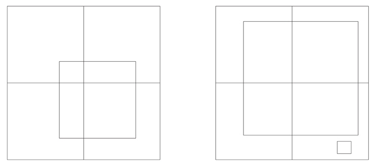
Not crucial but convenient is window specification, which allows a given data file to serve for experiments on a variety of CMD sub-regions. Data windows now are defined by the corner coordinates of rectangles, although only minor revision will be needed to permit more general shapes.

ADA is not 1. a substitute for good astrophysical modeling (it requires an embedded evolution model - any such model may need improvement); 2. for getting close, where experience is still needed. Automated “getting close” schemes certainly can be developed, but lie in the future.

So ADA is for follow-up on numerical experimentation, fine tuning, impersonal results, standard error estimates, and correlation coefficients. Future astrophysically informative experiments include analysis of several regions within a globular cluster. Usually those will be similar enough for one set of starting parameter values to serve for all regions, so preliminary experimentation need be done only once. In any case, the direct program makes experimentation easy. ADA currently has the following two problems:

I. it requires ultra-fast evolutionary computation (options are limited at present);II. its present evolution subroutine produces outlier CMD’s, even around the main sequence turnoff. Interpolation in tabulated evolution tracks offers a remedy.

Information on a cluster’s evolutionary state and history resides not only in the form of its CMD distribution, as conceptualized in the familiar wire-like isochrone, but also in the number density of stars within the form. This point is well recognized (e.g. Tolstoy & Saha 1996, Dolphin 1997, Vandenberg 2000), but the kind of analysis described here differs in major ways from all others, for example by direct inclusion of multiple star systems and by generation of standard errors and parameter correlation coefficients. It is specifically geared to impersonal extraction of numbers such as age, metallicity, and binary fraction.

Furthermore, not only does number density vary along the form, but the form is not one dimensional - its sequences have intrinsic widths for several reasons and are not symmetrical in width because of multiple star systems. The isochrone notion could be generalized to encompass the whole distribution, but that is not its ordinary meaning, so ADA essentially abandons the isochrone idea. The Least Squares criterion allows a variety of choices for the solution scheme (e.g. DC, Simplex, Steepest Descent, many others). Consideration of these points indicates CMD Areal Density, 𝒜, as the logical observable quantity for analysis, by standard Least Squares.

In comparison with other schemes for reaching a solution, DC has attractive characteristics of fast convergence, straightforward generation of correlation coeffcients, and standard error estimates that come from the covariance matrix in the usual way and do not require auxiliary numerical experiments. Its iterations can lead into a local minimum of variance that may not be the deepest minimum, but other solution algorithms have the same problem. Practical counter-measures are willingness to re-start from several points in parameter space and good intuition for starting points. ADA’s version of DC solves a main parameter set and any of its subsets for the same computational cost as for the main set alone, thereby allowing easy changes in the fitted parameters as a solution progresses. DC is well tested, with astronomical applications at least as far back as the 1930’s, and its operation within ADA is explained in Wilson (2001) and WH03. Other minimization algorithms would be satisfactory for ADA but do not produce standard errors and correlation coefficients. Most alternatives also are slower overall than DC, due to slow convergence.

The call to an evolution subroutine is only one program line within DC so that part of the ADA engine is easy to change. Of course the evolution routine must not only be accurate and reliable, but also very fast, as enormous numbers of stars are to be evolved. Why are so many stars evolved?

1. The number of stars to be evolved is large even for sparse clusters, as it is set by the requirement to have accurate theoretical areal density, not by the number of observed stars.2. Multiple star systems consist not merely of some number of stars, but have mass distributions that must be represented by a reasonable number of points. Five points on each companion mass ratio distribution have been used in experiments to date. The program distinguishes close from wide binaries, although that may be an unnecessary refinement in practice because of the relative rarity of close binaries, so altogether 11 stars may need to be evolved (1+5+5) for each primary on the Initial Mass Function (IMF). If only single stars and wide binaries are modeled, then only 6 evolutions need be carried out for each primary.3. DC requires evaluation of numerical derivatives (∂𝒜/∂p, where p is a parameter), so we need not just one evolutionary contribution to 𝒜 but (np + 1) contributions per star system, as a given system contributes once for each residual, 𝒜o - 𝒜c, and np times to form np partial derivatives.4. A parameter that affects evolution has a distribution in a real population and may need one in a solution. For example, metallicity Z might be assigned nZ values on each side of a Gaussian distribution plus a center value, thereby multiplying the number of stars to be evolved and the corresponding computation time by 2nZ+1. A parameter that is unrelated to evolution, such as interstellar extinction, may also be assigned a distribution, but with little effect on computation time.5. Parameter solutions are iterative, with typically of order 10 iterations per solution. Readers may wonder how areal densities and their derivatives can be stored for millions of theoretical systems (with binary and triple star distributions, metallicity distributions and error distributions) and thousands of pixels. Memory is economized if ADA only accumulates the contributions to 𝒜 for each system and each pixel. The contributions associated with each IMF primary are added to the 𝒜's for all pixels (most pixel contributions for a given system being zero, of course), and the memory arrays for system-specific quantities are then overwritten for the next IMF primary.

The present version of the ADA DC program can adjust any combination of the following 20 parameters, although experimentation has mainly been limited to subsets of six or fewer. The parameters are:

Z(fractional abundance by mass of elements 3 and higher);Gaussian standard deviation of Z;AV, interstellar extinction in V (or other vertical coordinate magnitude);Gaussian standard deviation of AV;Ratio of AV to color excess in B-V (or another color index);Intercept Aclose in mass ratio proba bility law Pclose = Aclose + Bcloseqclose for close binaries (q is mass ratio);Slope, Bwide, in above distribution;Intercept Awide in mass ratio probability law Pwide = Awide + Bwideqwide for wide binaries;Slope, Bwide, in above distribution;Reimers mass loss parameter η (winds);Binary enhanced mass loss parameter (Tout & Eggleton 1988);Lowest mass for which the IMF is defined;Mass at the first of two breaks in the IMF;Mass at the second break in the IMF;Exponent (of mass) in the Kroupa, et al. (1993; KTG) IMF for low mass stars;Exponent (of mass) in the KTG IMF for intermediate mass stars;Exponent (of mass) in the KTG IMF for high mass stars;Cluster V band distance modulus, V - MV;Cluster age, T;Number of stars above the low mass IMF cutoff (in the sampled part of cluster), Nstars.

The six parameters for which there is a significant basis in experience are Z, A_V, A_wide, V − M_V, T, and N_stars. The Z, A_V, and binary mass ratio distributions are not handled by Monte Carlo techniques but by the far more efficient Functional Statistics Algorithm (FSA), which is explained in Wilson (2001) and WH03. FSA achieves the statistical aims of Monte Carlo without random numbers, and its efficiency keeps typical ADA iterations within the range of 15 to 30 minutes rather than the days to weeks that would be needed under Monte Carlo.

Regular pixel structure provides a simple means of binning data in two dimensions, although quantization problems can defeat the overall goals if binning is too simplistic, so the imprint of pixel structure should be reduced as much as possible. Theoretical areal densities should vary smoothly from pixel to pixel, but much more important for solution stability is that DC’s numerical derivatives not be unduly affected by pixel quantization. The CMD dots that represent star systems can be visualized to be in motion through the pixel structure as parameters (p) are varied, and DC’s derivatives ∂𝒜/∂p are supposed to quantify that motion. However the contribution of a star system to the various ∂𝒜/∂p’s will be zero under simple binning unless the dot crosses a pixel boundary, in which case there will be a discontinuous jump. Of course DC’s residuals, δ𝒜 = 𝒜_o − 𝒜_c, also will be adversely affected. The numerous zero contributions with occasional big jumps may tend to average out for pixels with thousands of stars, but certainly they introduce enormous noise. However that noise is avoidable through pixel sharing, which leads to proper contributions to ∂𝒜/∂p for within-pixel motion and completely eliminates boundary-crossing discontinuities. In its simplest version, pixel sharing replaces the dot of ordinary binning with a plotting element that has the size and shape of a pixel. Theoretical 𝒜's thereby become smoother and their derivatives become entirely free of noise due to boundary crossings, thus greatly improving solution convergence and stability.

KTG recommend a mass function in three regimes (i.e. low, medium, and high mass), with each regime characterized by a specific exponent, denoted by p. ADA’s generation of zero age primaries is by uniform spacing of n_bin stars within a given mass bin in each of the three regimes according to

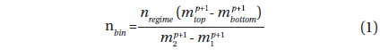
where n_regime is the number of stars in the mass regime, m₁ and m₂ are the regime boundaries, and m_bottom and m_top are the bin boundaries. A serious quantization problem can arise because, although the formula predicts n_bin as a floating point number, the actual number of stars to be evolved must be rounded to an integer. Consequences will be that the stars thereby evolved do not fairly represent the IMF, and that jumps in 𝒜 can occur as parameters p and N_stars vary. The situation is somewhat complicated, as each of the many combinations of primaries and companions can evolve to its own CMD pixel. The fix-up is to record the ratio of rounded to unrounded n_bin’s and correct the appropriate 𝒜’s separately for each system and its (up to 4) pixels. These corrections can be very important, especially where mass bin counts are low, but the corrections effectively compensate for IMF quantization.

An obvious difficulty is that open clusters typically have fewer stars than one would like for good statistics, with the relevant parameter being N_stars, as defined above. Although nothing can be done to improve the observational situation, theoretical counts can be increased by spacing stars more finely on the IMF and thereby increasing their number by a re-scaling factor 𝒜 that can be made large enough for theoretical 𝒜’s to be precise. Division of directly produced 𝒜’s by ℛ then produces correct 𝒜’s. The practical limit on ℛ will be set by computation time, so the idea is to have the product ℛN_stars large enough for departures from smoothness in pixel 𝒜’s to be unimportant. The opposite difficulty can be encountered for globular clusters, where N_stars may be large and lead to excessive computation time. The simple expedient is to set ℛ smaller than unity for rich clusters, and perhaps even much smaller. Given that the observations are definite and need only minor computations, overall computational needs are set by the requirement of having smooth theoretical 𝒜’s, which ℛ can control.

Computional efficiency can be improved by recognizing that statistics are far better for low than high mass stars, due to the steepness of the IMF. Suppose the number of theoretical stars to be evolved is very large, perhaps because the re-scaling factor ℛ is something like 100, or perhaps just because N_stars is large. Without further action, the number of low mass stars will be extremely large. An ultra-simple remedy could be to have the same number of stars in all IMF bins and then convert the resulting 𝒜 contributions according to a realistic IMF, but there is a better way - the situation is made more flexible by operating with a fictitious IMF, to generate theoretical stars, in addition to the real physical IMF. A correction for each IMF bin is easily computed, tagged onto each star system, and subsequently used to correct its 𝒜 contributions to the appropriate CMD pixels. For example, WH03 adopted exponents p_1,2,3 = −0.30 for all three IMF regions in generating theoretical stars and then corrected each star’s 𝒜’s to what they would be with KTG’s recommended exponents of p₁ = −1.3, p₂ = −2.2, and p₃ = −2.7. The same exponents were used for this paper’s experiment.

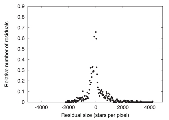
Justification for the Least Squares fitting criterion is based on distributions of observables being Gaussian and the method works best when that is realistically the case. Fig. 1 shows a distribution of residuals for ADA pixels.

[Fig. 1.] Typical distribution of ？ residuals. Each dot represents a pixel.

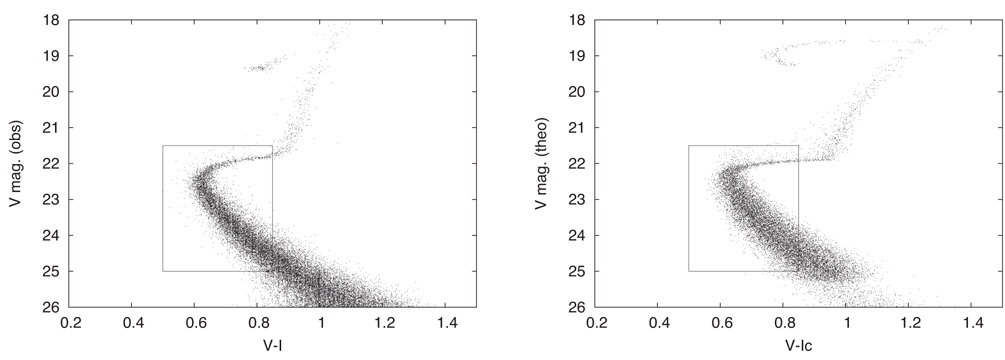
Note that the distribution is significantly asymmetrical, as is most easily seen by comparing its two tails. The reason is that areal density is logically positive, so observed ADA is capped at a lower value of zero but is not capped at any definite upper value. Theoretical ADA’s have been made as smooth as we can manage via the schemes discussed above (pixel sharing, re-scaling, rounding within mass bins) so they have neither large positive nor large negative excursions, therefore having small positive values in lightly populated pixels. Statistical fluctuations of the observed areal densities thereby make a long tail on the positive residual side that is not matched on the negative side. Suppose one were apply pixel sharing to the observed points. In ordinary pixel sharing where the plotting element has fixed size, the δ𝒜 distribution can be made more nearly symmetrical by use of larger pixels, thereby smoothing the 𝒜_o’s, but at the cost of diminished resolution in high density areas where asymmetry of δ𝒜’s is not a significant problem. The general remedy is to have the plotting element size vary with CMD location, being large in low density areas and small in high density areas. An optional refinement on DC’s pixel sharing has been to allow the plotting element for observed points to be larger or smaller than a pixel, a feature that can make residual distributions more nearly Gaussian while preserving resolution. The acronym is VDF, for Variable Density Factor, with the local VDF based on a pixel’s observational counts. Where the plotting element turns out to be small (high density pixels), it is nearly like plotting a dot for an observed point (see Fig. 2), so loss of resolution is negligible in high density regions.

[Fig. 2.] Illustration of plotting elements for ordinary pixel sharing (left) and Variable Density pixel sharing (right). The main purpose of pixel sharing is to allow accurate numerical differentiation of areal density with respect to solution parameters. Variable Density pixel sharing operates with large plotting elements in low density areas for good averaging, and small elements in high density areas for good resolution. Although the larger illustrated element is only modestly larger than a pixel, actual situations may call for very large elements.

DC iterations can diverge, although that is true of many iterative Least Squares solution algorithms. The problem is not ordinarily caused by inaccurate derivatives, ∂f/∂p (where f is an observable function and p is a parameter), but by absence of second and higher derivatives in usual formulations, coupled with parameter correlations. In pictorial terms, standard DC tries to traverse a curved surface in multi-dimensional parameter space by linear algebra. That will work in short steps, but correlations can lure DC into taking long steps. Introduction of higher derivatives usually is not feasible, especially if one considers the need for cross-derivatives, ∂²f/∂p₁∂p₂. Maintainance of good accuracy in numerical second derivatives also is difficult.

A very effective way to combat the problem is the Levenberg-Marquardt (L-M) scheme (Levenberg 1944, Marquardt 1963), which effectively merges DC with the Steepest Descent solution method so as to exploit the best convergence characteristics of both. With w written for weight and r for (observed - computed) residual, the Method of Steepest Descent examines the local variance, Σwr², and follows its negative gradient. Steepest Descent can be very slow but is resistant to convergence troubles, whereas DC’s convergence is fast but trouble is a possibility. Marquardt (1963) introduced a (typically small) parameter λ that is added to each diagonal element of the normal equation matrix after the equations have been rescaled so as to have diagonal elements of unity (so the diagonal elements become 1 + λ). Marquardt also gave an intuitive view of the merged scheme, whose iterations are fast and greatly improved in reliability. Some authors continually revise λ as a solution progresses, with the aim of reducing it to zero at the end, but experiment shows that a very wide range of λ (say 10⁻⁴ to 10⁻¹⁰) gives essentially the same parameter corrections, regardless of whether the operating point is close to or far from the Least Squares minimum. Accordingly, λ was 10⁻⁵ throughout the iterations of this paper.

Another very good way to strengthen convergence is the Method of Multiple Subsets, or MMS (Wilson & Biermann 1976), whose idea is to simplify the correlation matrix by breaking it into smaller pieces. Correlations are not necessarily smaller under MMS, but DC needs to deal with fewer correlations. As before, the Least Squares problem must cope with non-linearities, correlations, and many dimensions. The MMS strategy is to reduce the number of dimensions and thus reduce overall complexity. All that need be done is to operate with some number of subsets of the full parameter set. For an example with six parameters, DC might alternate between two subsets of three parameters each. There seems to be a misconception that the MMS may be needed away from the Least Squares minimum but not at the minimum (De Landsheer 1981). However that is not true - if MMS is needed, it is needed all the way, including exactly at the minimum (Wilson 1983).

Sometimes neither L-M nor MMS is needed and sometimes one or the other is enough, while especially difficult situations require both. The two schemes are in ADA’s DC program, which includes L-M in the way mentioned above, and MMS via the option of multiple subset solutions as part of each program submission.

The various CMD sequences and branches (e.g. main sequence, subgiant branch, etc.), and of course the CMD as a whole, will differ statistically between observation and theory if noise is omitted from theory. Theoretical patterns will be too narrow and there will be no chance of a meaningful match if this issue is ignored. Photometric errors enter the problem differently than do statistical star count fluctuations. Star count statistics appear as δ𝒜 fluctuations, whereas photometric errors show up as wrong CMD locations, perhaps in the wrong pixel, so the pattern broadenings discussed here are caused by photometric errors. Photometric noise has several essentially Gaussian sources such as sky transparency variations and photon counting statistics (both simulated in the present ADA model), with the latter dominant in magnitudes and color indices of faint stars. Errors due to unresolved optical multiples also change CMD locations and have distinctly non-Gaussian statistics. The analogous pattern mis-match situation in ordinary x,y graphs is uncommon, but that is because many x,y problems that involve counts (and therefore bins) have time as the “x” variable, and time can be measured very accurately. If not time, then frequency or wavelength (also measured precisely) may be the “x” variable, so pattern mis-matches tend to be unusual in x,y fitting and may seem characteristic of higher dimensions. In reality the mis-matches are un-related to dimensionality. Accordingly, ADA needs to model photometric errors and apply them to CMD locations. A model parameter (or more than one) is needed for noise in each photometric band - for example two parameters for V vs. V-I. A convenient choice is the set [N_V=0 ; N_I=0], the numbers of photon counts for a star of zero magnitude in each observed band.

[Fig. 3.] Comparison of an observed test case (left) and the ADA fit (right) in V vs. V-I. The CMD’s are shown side by side rather than in one panel to avoid need for a plot in color. Agreement is not very good due to deficiencies in the adopted theoretical evolution tracks, although there was strong convergence to a definite solution. Use of tabulated evolution tracks will fix this problem. The boxed region is the fitting window.

How can photometric noise be made part of the model? As we are dealing with distributions (in this case, error distributions), an efficient way is via FSA, as explained in Section 3 of Wilson (2001) and Section 6.3 of WH03, where 9 × 9 distributions were applied (9 magnitude errors, 9 color index errors). Error distributions require little computation time because no evolution is involved and because the Gauss error function (ERF) that computes the abscissas needs to be entered only a few times, as that computation is the same for every star system. Only very modest memory allocation (9 × 9 × 36 = 2916 in WH03’s example with binaries and triples) is required for theoretical magnitudes and colors, with each IMF primary represented by 36 star systems of various mass ratios - a single star, 10 binaries, and 25 triples. For this paper’s example with only single stars and binaries, there are only 6 star systems for each IMF primary.

The convergence situation is almost entirely good. From a reasonable intuitive start, one or two iterations often are enough to reach the essential answers, after which typically 5 or 6 refinement iterations reach a stable Least Squares minimum. Sometimes minor jiggles continue, but ordinarily they are well below levels of astrophysical significance. Causes of small jiggles may be essentially discontinuous evolutionary events, such as red giants becoming white dwarfs and jumping from one CMD location to another. Note that red giant to white dwarf transitions can be a problem from the side of theoretical modeling even with no red giants in the window when a red giant has a companion. Whereas a single red giant that is well outside the CMD window typically jumps to another place outside the window upon becoming a white dwarf, one with an unevolved or mildly evolved companion can easily jump into the window, thus suddenly appearing “from nowhere” and causing discontinuous Areal Density behavior. That is - the giant effectively disappears but the companion is still there. Fortunately such events have been rare in experience to date, but one should recognize their existence and be alert for corresponding convergence degrradtion.

Three iterations from the middle of a solution are tabulated below so that readers can have a partial experience of examining the overall process. The preceding DC iterations began from a fit that was found subjectively (trial and error) and subsequent iterations went on until all corrections were smaller than the standard errors, including a few iterations at the very end to be sure that the operating point was not creeping slowly along (i.e. that the corrections were not consistently of the same sign). Convergence in iterations 3, 4, and 5 is almost at the final stage where corrections (column 3) are small compared to the standard errors (column 5). Departures from perfect arithmetic in the iterations are due to rounding in making the tables.

With these refinements, DC can find a Least Squares solution very accurately, as shown by Fig. 2 to 6 of WH03, where there is no discernable departure of derived parameters from the Least Squares minimum. Each illustrated curve was computed with 5 of the 6 parameters at the solution value, and the weighted variance was generated as the other parameter varied.

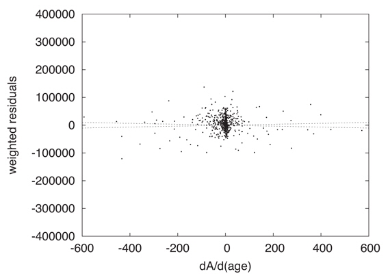
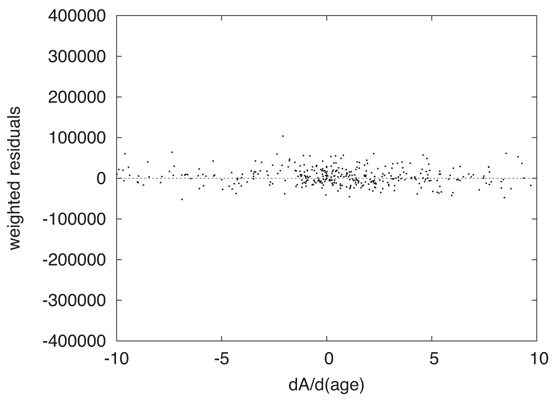
Graphical examination of actual Least Squares problems solved by DC helps one to explore parameter uncertainties intuitively. Figure 4 shows observed minus computed residuals, 𝒜_o − 𝒜_c, graphed vs. cluster age (T) derivatives, ∂𝒜c/∂T. Each dot is for a pixel, and both the residuals and the derivatives were weighted according to the inverse variance of the photometry. The figure isolates one of the 6 parameter dimensions and is for a converged solution, so it corresponds to the end of an iterative process in which the machine has successfully made the residual distribution flat. That is, DC has searched for a solution in which the residuals are uncorrelated with the derivatives. The widely distributed points mainly represent the subgiant branch. Readers will notice a dense concentration of points near the origin, which are main sequence and turnoff region pixels. There the ∂𝒜_c/∂T’s are small because evolutionary motion is very slow and the residuals are small because the large numbers of stars lead to good statistical averaging. Fig. 5 magnifies the region around the origin and shows that flatness has been attained there also, so the fit for the main sequence turnoff is also a solution for the entire CMD window. Such diagrams for the other five parameters also are flat for this solution so DC has achieved its goal according to eye inspection. These two figures include what might be called 1σ lines. The horizontal axis represents the solution and the 1σ lines correspond to the solution being off by ±1 σ_T, thus giving a visual impression of the uncertainty of fitting. In this solution and others, one can imagine trying to fit a horizontal line by eye, judge how well the machine has done its job, and look for irregularities and inconsistencies.

[Fig. 4.] One dimension (cluster age) of the 6 dimensional Least Squares solution in graphical form. DC seeks to make the residuals uncorrelated with the derivatives (flat distribution). The slightly diverging straight lines are 1σ age limits. See text for further explanation.

[Fig. 5.] A detail of the inner core of points in the preceding graph. These are main sequence and turnoff region pixels. The 1σ age limits are shown again, but their divergence is too small to see over such a small range of the abscissa.

Much work with clear goals remains on evolutionary accuracy. The idea is to develop fast versions of evolution programs by a mix of approximation functions and tabular interpolation, and to allow variation of important parameters that have fixed values in the one fast evolution program now embedded in the ADA programs. Those parameters characterize mixing length in superadiabatic convection zones, convective overshooting, helium abundance, specific abundances such as “α” elements O, Ne, Mg, Si, S, and Ar, and other physical conditions. Future ADA applications will allow selection among numerous fast evolution subroutines developed by various persons. Armed with such an ADA program and having arrived close to a solution, whether by a future automatic algorithm or by trial and error, one will carry out impersonal solutions according to several or all of the evolution routines. This is where the labor saving characteristic of ADA will show to best advantage, as one has to get close only once, whereupon the machine can take over.

So the main problem areas are evolutionary accuracy and need for further adjustable parameters. Otherwise ADA works well. Simulations show that solutions for cluster age, binary fraction, distance modulus, metallicity, and interstellar extinction recover known results from synthetic clusters when the same evolution model is used for simulation and solution. Convergence of the iterative solutions is usually fast and gives essentially stable final results, accurately at a Least Squares minimum in multidimensional parameter space. Correlation matrices show that overall correlation problems tend not to be unduly severe. Typically most correlations are within ±0.2 or so, perhaps with a few around ±0.6 to ±0.7, and with none close to unity, although experience to date is limited to 6 or 7 parameters. The routines that convert observable flux and temperature to magnitude and color index have been thoroughly tested and are reliable, although now limited to 25 standard photometric bands.