The atmospheric flow in the 3-Cell model of global atmosphere circulation is described by the Lagrange's equation of the non-inertial frame where pressure force, frictional force and fictitious force are mixed in complex form. The Coriolis force is an important factor which requires calculation of fictitious force effects on atmospheric flow viewed from the rotating Earth. We make new Mathematica platform to solve Lagrange's equation by numerical analysis in order to analyze dynamics of atmospheric general circulation in the non-inertial frame. It can simulate atmospheric circulation process anywhere on the earth. It is expected that this pedagogical platform can be utilized to help students studying the atmospheric flow understand the mechanisms of atmospheric global circulation.
Motion observed on the rotating Earth is generally explained by invoking inertial forces described in the noninertial frame of reference (Symon 1971, Landau & Lifshitz 1976). Because viewing the motion from accelerating or rotating frame of reference introduces fictitious forces added to actual forces. On account of the inequality in energy absorbed at a spherical surface of the rotating Earth, seven zones of atmospheric pressure are formed over the Earth surface: an intertropical convergence zone (ITCZ) near the equator, two subtropical highs in both Hemispheres at the latitude of 30°, two subpolar lows on both Hemispheres at the latitude of 60°, two polar highs on both poles. Accordingly, global scale circulation of the atmosphere is described by the Lagrange's equation in the non-inertial frame of reference according to the 3-Cell general circulation of the atmosphere (GCA) model rather than Hadley Cell model (Ahrens 2001). Long-term recording data from the satellites approve of the 3-Cell GCA model (“AMNH-Weather and Climate Events” 2014, “Global Climate Animation” 2014). On the rotating Earth frame, the Coriolis force acts as a most important force to change the direction of surface airflows on the Earth. The deflection is not only instrumental in large-scale atmospheric circulations, the development of tropical cyclones, hurricanes and typhoons, also it can affect missile launching, satellite operation, and GPS position sensors (Bikonis & Demkovicz 2013) in the modern sciences. Effects upon the weather, ocean currents, rivers and projectile motions are well documented (Graney 2011, Mclntyre 2000), but the motions over very long distance are required for discernible effects. Common pedagogical tools are helpful to explain the Coriolis effects. For example, Merry- Go-Round table (“Merry-Go-Round” 2014) or Bath-Tub Vortex (Trefethen et al. 1965) is helpful for explaining the Coriolis effects, but it cannot be distinguished whether its effect is from Coriolis force or centrifugal force unless we calculate the forces with their vector components. While this approach simplifies some problems, there is often little physical insight into the motion, in particular, into the fictitious force of the vectorial characteristic.
Recently, efficient visualization programs are utilized for the Coriolis force effects (Zimmerman & Olness 1995, Tam 1997, Yun 2005, Zeleny 2010). In particular,
2. LAGRANGE’S EQUATION IN A NON-INERTIAL FRAME OF REFERENCE
In the inertial frame, space should be homogeneous and lime is isotropic to assert the invariance of the mechanical sysrem. If we were to choose an arbirrary frame of reference, space would be inhomogeneous and anisotropic. Therefore, the equation of motion in the rotating Earth system should be described in the non-inertial frame ofreference (Landau & Lifshitz 1976). For the validity of the principle of least action in the mechanical system independent of the frame of reference chosen, we must carry out the necessary transformation of the Lagrangian Lo for the Lagrange's equation in the non-inertial frame of reference. This transformation is done in two steps. Firstly, we consider a frame of reference K' which moves with a translational velocity relative to the ineltlal frame Ko. Next, we bring a new frame of K which rotates relative to K' with angular velocity, . As a result, K executes both translational and rotational transformation to the inertial frame Ko (fix star):. The Lagrangian in Ko frame is (Landau & Lifshitz 1976)

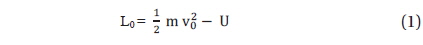
where, Vo is the velocity of a particle in Ko frame and U is a potential. The velocities come from a transformanon and the come from a transfonnation Finally, me Lagrangian in K frame is
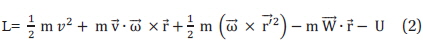
where, Then Lagrange's equation, which satisfy the principle ofleast action,
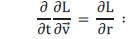
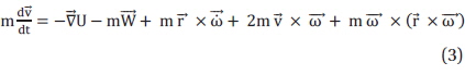
If we suppose that angular velocity is constant and neglect dle translational velocity, we omit and . Then Eq. (3) is

We rewrite this again as

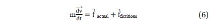
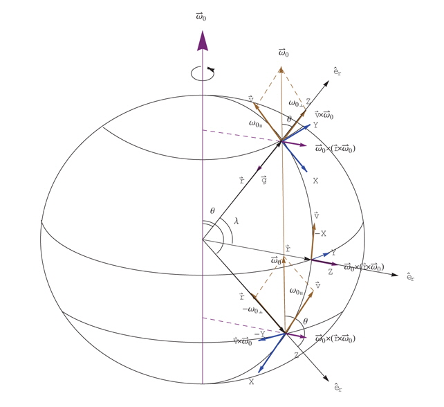
This is just a Newton's equation, which shows the motion of an object by the force Here includes the friction and the pressure gradient force. and the includes the CorioHs force 2m wand the centrifugal force m( ) ×() which deflect the atmospheric flows on the rotating Earth. As shown in Fig.1, the CorioJis acceleration vector direct to ±Y direction. Deriving process of the Lagrange's equation in the non-inertial frame is well described in other books (Symon 1971. Landau & Lifshitz 1976).
3. MATHEMATICA PROGRAMING FOR GERNERAL CIRCULATION OF THE ATMOSPHERE
3.1 Vector calculation of the effective force
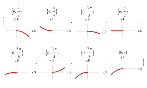
To analyze the deflection effect of the atmospheric flow based on the 3-Cell GCA model at any point on the Earth's surface, we create a position function point[t, θ] in solving the Eq. (4) in
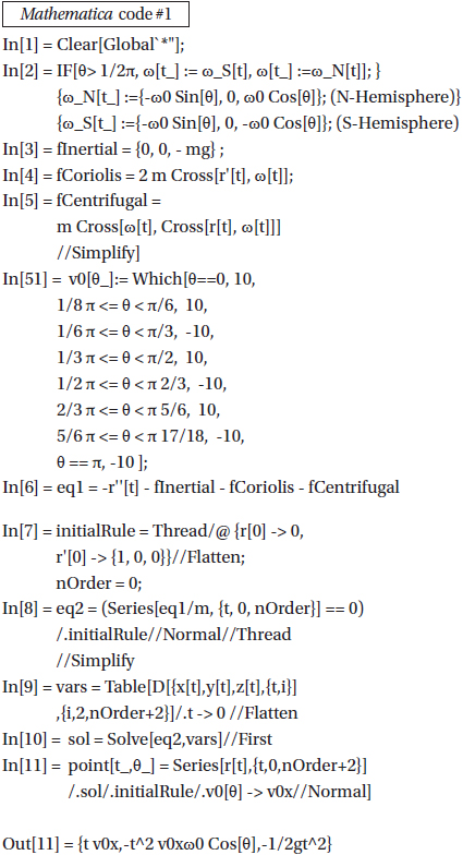
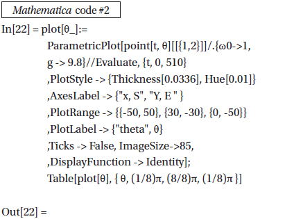

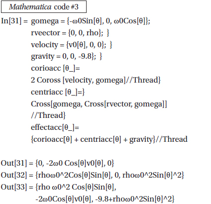
However, Fig. 2 does not show which fictitious forces cause the deflections unless we calculate those with their vector components respectively. Because the deflections of the winds over the globe come from the resultant effective force in Eq. (5), we must calculate accurately the ingredients of the effective force for the probable cause of deflections. For the examination of the deflection effects of the effective force, we calculate the constituent parts of the effective force accelerations with its vector components at the eight cities respectively, and summarize those in Table 1. The vector calculation of the fictitious forces with those components is easy in
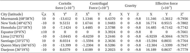
The accelerations of the effective force calculated with those vector components at the eight cities. The calculation parameters: ω0 = 7.292 × 10⁻⁵ sec-1, g=9.8 m/sec2, and the unit of the acceleration is m/sec2. Minus sign of the stands for the wind direction to the north unit of m/sec.
3.2 Mathematica platform for the 3-cell atmospheric general circulation model
Understanding the vectorial nature of the effective forces on the Earth's surface is a keyword of the atmosphere circulation dynamics. However, it is not easy to evaluate the wind deflection effects at any point on the Earth's surface, because the deflection is varying on the resultant wind vector and associated effective force vectors at the point belong to the atmospheric pressure zone matching to 3-Cell GCA model. The fundamental concept of the inertial force effects in the non-inertial frame of reference is essential to analyze the GCA dynamics. Visual representation of such vectorial nature of the GCA will be in valuable to the researchers working in this field and help teach physics or meteorology students.
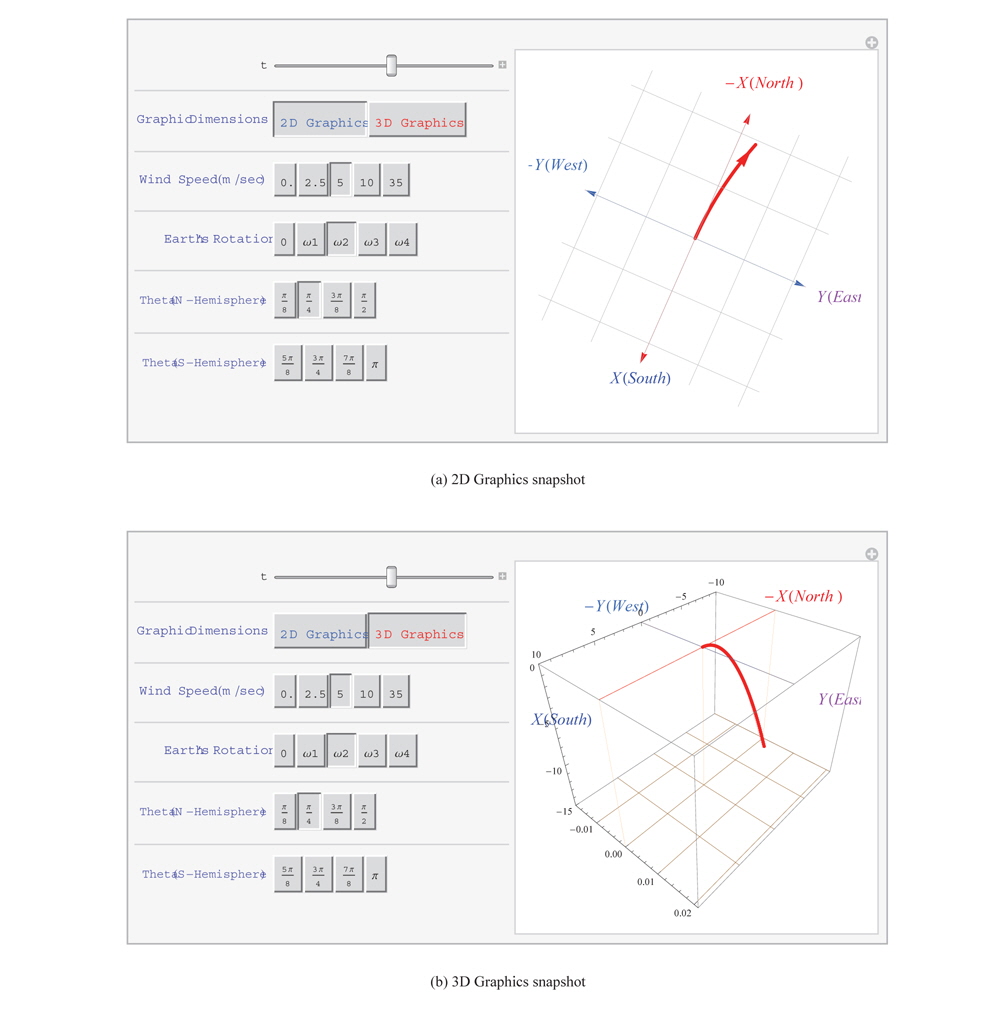
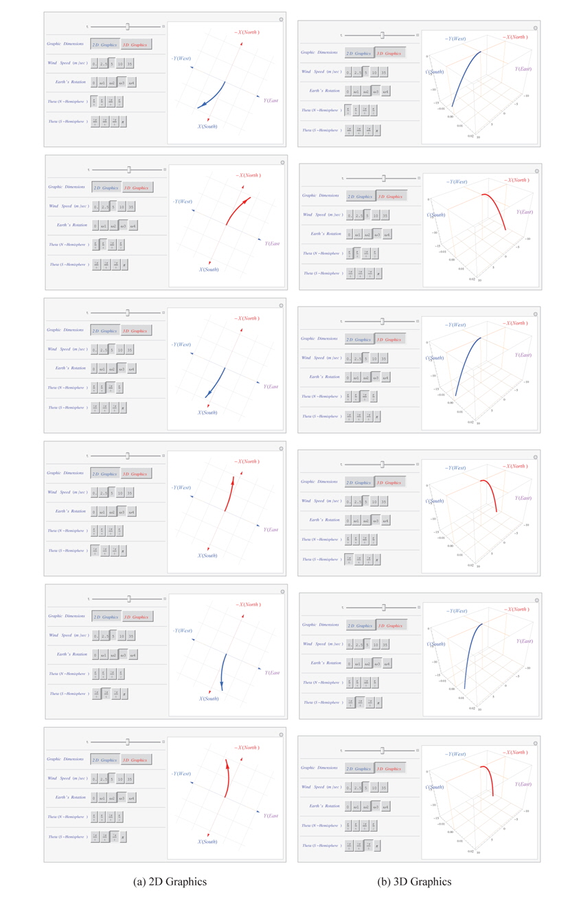
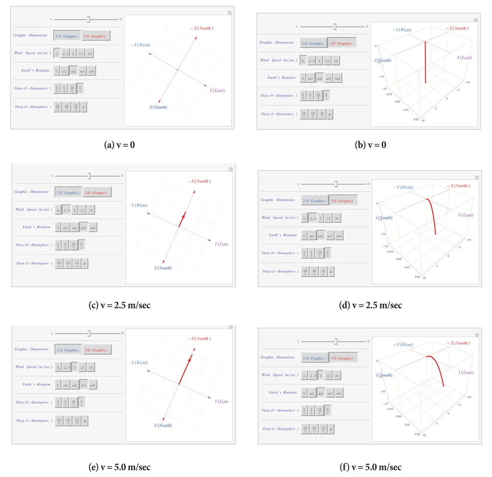
We provide Coriolis effects platform to simulate the wind progressing on the rotating Earth's surface matching the 3-Cell GCA model using the function Manipulate in Mathematica. Fig. 3 a is a 2D Graphics snapshot of the platform and Fig. 3b is a 3D Graphics snapshot of the platform. The platform draws the path of the wind through the point[t, θ] with a time domain of vector array of the solution of Eq. (4) using the Parametric Plot of Mathematica. On starting the program, platform will show Fig. 3a. Simulation performs the built-in program when you click the ► appearing while you spread the ⊕ of
The Earth is a planet of a sphere which revolves the fix star while rotating itself with a constant angular velocity. The frame of reference on the rotating Earth is a non· inertial frame of reference since the frame is in acceleration continuously. Therefore, the equation of motion should be modified through the coordinate's lransformarions by the least action principle in the mechanical system of Eq. (4): Here the Coriolis force 2 m wand centrifugal force m × () are the most important fictitious forces which play a significant role in a variety of natural processes, most prominently the atmospheric circulation dynamics. In particular, the Coriolis force is also responsible for the circular motion of the tropical cyclone, the tropical typhoon and the hurricane. Physical comprehension and manifesting ability for the non-inertial frame of reference on the rotating Earth becomes a merit of asset to physicist and natural scientist. The conception of the inertial forces on the Earth has been recognized recently because the Coriolis force is not only the most important effective force in the GCA dynamics but also an indispensable task for the scientist in long-range missile launching, satellite operation and GPS position sensors in modern technology. We demonstrate the Coriolis effects platform to simulate the wind progressing on the rotating Earth's surface matching the 3-Cell GCA model in