Topology optimization is one of the useful methods for finding the layout of an optimal structure in a given design domain for the load-bearing structures. Generally, because there are usually two or more loadings on a structure in a structural topology optimization problem, it becomes a multi-objective optimization problem [1]. In multi-objective optimization problems, solutions consist of a Pareto optimal set, which can only be improved by degrading at least one of its other objectives. The objective in solving multi-objective topology optimization problems is to find complete Pareto-optima solutions [2].
For the topology optimization, various methods have been developed [2-8].One popular approach for multi-objective topology optimization is the solid isotropic material with the penalization (SIMP) method (Bendsøe, 1989) using the weighted sum method [4]. The SIMP method redistributes the material throughout the specified design domain using an optimality criterion [3]. The SIMP method is extended to multi-objective optimization using the weighted sum method, because this method is relatively easy to implement and finds Pareto-optimal solutions quickly. However, the SIMP method has multiple optima because most topology design problems have non-convex objective functions [4]. Thus, it is difficult to find a single optimal solution. Moreover, the weighted sum method cannot find a complete Pareto-optimal solution set if the objective space is non-convex [2].
To perform global searching and find the complete Pareto-optimal set, genetic algorithms (GAs) have been increasingly used in the multi-objective topology optimization problems. In the GAs, individuals of the GA are evolved simultaneously by cooperation and competition. Thus, a GA can find Pareto-optimal solutions in a single simulation. However, because a GA requires a large number of evaluations of objective functions, its computational cost becomes high. This computational cost problem is the most important factor in optimization problems using GAs [8].
In this study, for an efficient multi-objective topology optimization method using a GA, the elite initial population method was proposed. The elite initial population which is similar to local optimum solutions obtained from the SIMP with the weighted sum method was used for the initial population of the GA. The SIMP with the weighted sum method can provide well converged and distributed individuals in the objective function space. A local optimum solution used as a good initial guess helps to improve the efficiency of the GA. In this study, to verify the convergence and diversity of Pareto-optimal solutions of the proposed method, a standard initial population and an elite initial population were compared.
2.1 SIMP with the weighted sum method for a multi-load case problem
In this study, local optimum solutions, which are obtained by SIMP with the weighted sum method, were used for an initial population of GA. In the SIMP with the weighted sum method, the problem of optimizing the structure topology for minimum compliance can be formulated in a discrete form as follows.


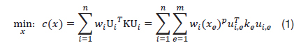
where C is the compliance,
In the SIMP using the weighted sum method, Pareto-optimal solutions can be easily obtained using a varied set of weights such that and wi > 0. The computational efficiency SIMP method is greater than a GA-based method, because it is a gradient-based method. However, The computational efficiency of the SIMP method is greater than a GA-based method, because it is a gradient-based method. However, if the objective function space is multi-modal (non-convex), the optimization problem has non-unique solutions when choosing different initial points and design parameters for the algorithm [4]. Moreover, although implementation of the weighted sum method is very easy, it cannot find complete Pareto-optimal solutions [2]. Conversely, the GA topology optimization can find complete Pareto-optimal solutions more effectively. However, it is necessary to reduce the computational cost [8].
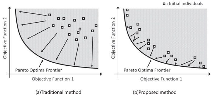
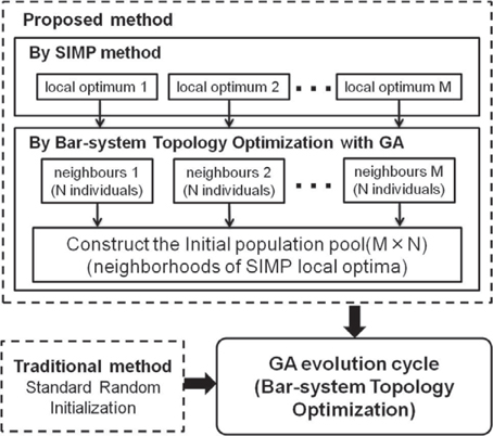
Therefore, in this study, local optimum solutions obtained from the SIMP with the weighted sum method, which is more computationally effective than simply using a GA, were employed for the initial population of the topology optimization to improve the efficiency when using a GA. Well converged and distributed local optimum solutions become good initial guesses for the GA, and lead to more rapid convergence to Pareto-optimal solutions as shown in Fig. 1.
Figure 1 shows illustrations of the traditional and proposed methods. Generally, in the traditional method for GAs, a standard random initializing procedure is used for the initial population. Its initial population is completely random as shown in Fig. 1(a). Conversely, the initial population of the proposed method already has well converged and distributed solutions, because local optimum solutions were used as initial populations as shown in Fig. 1(b). By comparing Figs. 1(a) and (b), the proposed method is expected to converge more rapidly than the traditional method.
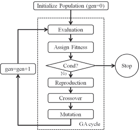
The flowchart of the proposed method is presented in Fig. 2 and summarized here:
1) Generate M local optimum solutions using the SIMP with the weighted sum method. 2) Create M×N individuals that have topologies similar to each M local optimum solution of Step 1 using topology optimization using the GA. 3) Randomly select L individuals obtained from Step 2 for the initial population of topology optimization using the GA.
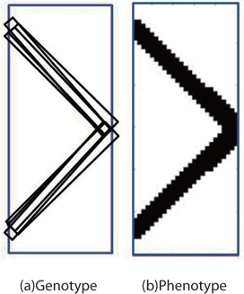
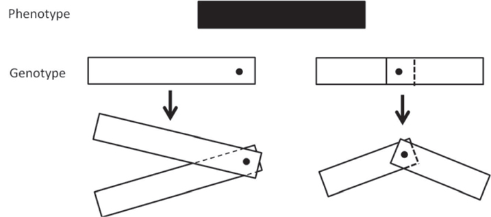
In topology optimization using the GA in Step 2 and 4, the bar-system representation method [8] was used for the topology representation. It is well known that the choice of a topology representation method is critical to the process. In the bar-system representation, the positions of the vertices and thickness of the bars are used as design parameters in the topology optimization using a GA. Mapping on the FE mesh is simple in the bar-system representation. If the center of gravity of that element lies inside bars, the density of the element becomes 1. Thus, the density of an element is only 0 or 1. Figure 3 shows the topology example for a bar-system representation. Figure 3(a) and (b) shows an example of the genotype (artificial chromosome) and phenotype (the decoded parameter), respectively.
However, it is difficult to use local optimum solutions directly for the initial population of a GA, because properly decoded GA genotype must be found, corresponding to local optimum solutions with bar-system representation. Thus, topology optimization using a GA was used in the Step 2 to create individuals corresponding to local optimum solutions. We called these individuals the “elite initial individuals”. However, it is difficult to find the elite initial individual with exactly the same phenotype as the local optimum solution. Moreover, there are many genotypes corresponding to one phenotype. Thus,
First, in the FEM element of the local optimal solutions of Step 1, if an element has a density below 0.05 it will be modified to -0.5. The densities of other elements remain as they are. However, if a volume constraint is introduced, it is not necessary to modify the density of any elements in this step. The density values 0.05 and -0.5 were determined empirically
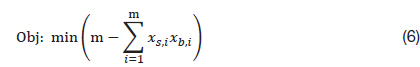
Second, to find the proper genotypes corresponding to the local optimal solutions, the density distribution of the modified local optimal solutions, and the phenotype transformed from the genotype using the bar-system representation, were compared in Step 2 topology optimization using a GA with formula (6) as the objective function.

where
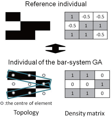
Formula (6) is used as the objective function of topology optimization using the GA of Step 2. However, the computational cost must be investigated. Because formula (6) is a simple sum of the products of a matrix, its computational cost will be low. We present an example of formula (6) as shown in Fig. 4. Because
3. Multi-objective optimization problem method using GA
3.1 Multi-objective optimization problem
Generally, a multi-objective optimization problem can be formulated in a discrete form as follows:
where f
3.2 Elitist non-dominated sorting GA with archiving
In the multi-load case problem, the elitist non-dominated sorting genetic algorithm (NSGA-IIa) [9] which is one of the best known Multi-Objective Evolutionary Algorithms (MOEAs), was used to minimize the compliance of each loadcase.
The flow of NSGA-II is similar to the flow of a common GA [10] as shown in Fig. 5. However, to improve diversity and convergence of solutions in this algorithm, the crowding distance metric and the crowded tournament selection are introduced. The crowding distance metric is the relative average distance to other individuals with the same rank in the objective space. The crowded tournament selection is used to compare two individuals and returns the winner of the tournament according to the rank and crowding distance between them. Moreover, an elitist strategy was applied to avoid the problem of losing Pareto-optimal solutions. If the number of Pareto-solutions exceeds the population size, some Pareto-optimal solutions can be eliminated. Therefore, an archiving method was used for the solutions preserving method. For the crossover method of a GA, the parent centric crossover (PCX) [11] and the binary-like crossover [10] methods were applied simultaneously, and for the mutation method of a GA, the polynomial mutation [12] was applied.
4. Verification of the proposed method
To verify the efficiency of the proposed method, a simply supported beam structure compliance minimization problem was used. In this section, the traditional and two proposed methods were compared to perform a comparative study as follows:
Method1: Standard random initialization method (Traditional method)Method2: 20×N elite initial population (Proposed method with M=20)Method3: 40×N elite initial population (Proposed method with M=40)
where
To verify the efficiency of the proposed method in the multi-objective topology optimization problem, the convergence and diversity were compared using the hyper volume ratio (HVR) and Pareto-optimal frontier. By using HVR, it was possible to provide a qualitative measure of the convergence and diversity of the Pareto-optimal solutions. Moreover, the computational cost of each method was compared to verify the efficiency of the proposed method.
4.1 Compliance minimization problem for the simply supported beam
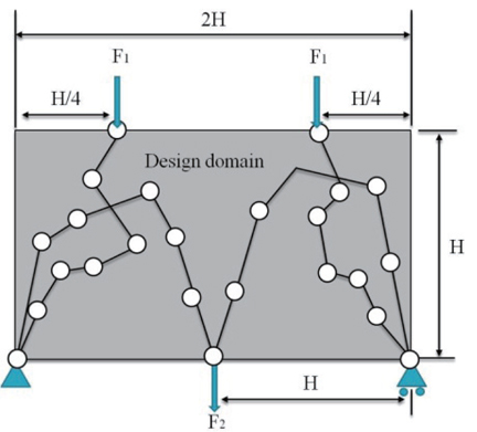
A simply supported beam structure as shown in Fig. 6. was adopted as the verification problem for the proposed method. Figure 6 shows the design domain and bar system of the structure. A design domain of 2H×H discretized into a 40×20 mesh was used, and the loadings F1=1 and F2=1 were assumed. The basic parameters assumed were Young’s modulus E=1.0, Poisson’s ratio
For the GA parameters of Step 2, a population size of 50, crossover probability of 0.9, and mutation probability of 0.2 were used. Total number of generations was 100. The optimization problem of topology optimization using a GA was to minimize formula (6).
On the other hand, for the Step 3 GA, a population size of 100, crossover probability of 0.9, and mutation probability of 0.2 were used. The optimization problem of topology optimization using a GA was to minimize compliances for the given two load cases of the structure with a 0.4 volume fraction.
Hyper volume is generally used for the qualitative measurement of convergence and diversity in a multi-objective optimization problem [2]. Hyper volume is constructed with Pareto-optimal solutions and a reference point in the objective space. The reference point was set as a vector constructed using worst objective function values. The metric HVR is usually introduced to calculate a normalized HV value. This HVR is the ratio of the HV of Q and of P* as follows.
where HV(Q) is the HV calculated for the Pareto-optimal solutions and HV(P*) is the maximum (ideal) HV value. When Q=P*, HVR=1. If Pareto-optimal solution convergence and diversity are improved, HVR is close to 1. For the calculation of HVR in this study, the results of Method 1 with 600 generations, Method 2 with 300 generations, and Method 3 with 300 generations were used as the ideal HV(P*), because generally the ideal HV(P*) of a formula (8) is not obvious.
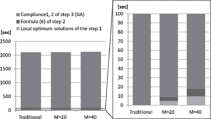
Table 1 shows the average number of evaluations of the objective function per single GA trial and the average evaluation time of the objective function per single evaluation. In Table 1, the average number of evaluations of compliance was calculated, because the SIMP with weighted sum method of Step 1 was used until convergence and might have obtained different solutions if choosing different initial value. Because the GA in Step 2 was implemented up to 50 generations with 100 populations, the number of evaluations of formula (6) at Step 2 can be calculated as 50 (total number of generations) × 100 (population) ×
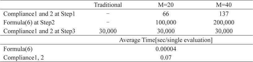
Average number of objective function evaluations per single GA trial and average evaluation time for the objective function (40×20 meshed beam) Originals of tables used in the text (each on a separate sheet).
Computational time
In the case of the 40×20 meshed model, formula (6) and compliance 1, 2 average calculation times were 0.00004 and 0.07 s, respectively, and all the CPU times were measured on a desktop computer with a 2.8 GHz Intel Core i7 processor clock speed.
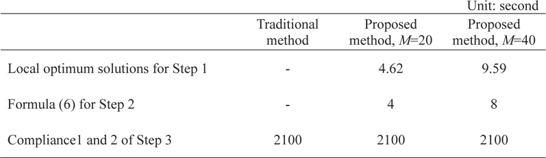
Table 2 and Fig. 7 show the total computation time for each method (methods 1-3). As shown in Table 2 and Fig. 7, the additional computation times for the proposed method (the cost of Steps 1 and 2) for
5.2 Convergence and diversity of Pareto-optimal solutions
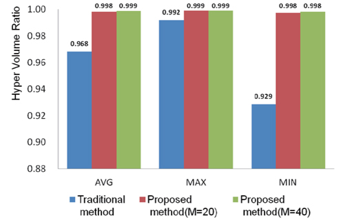
In this study, to verify the convergence and diversity of Pareto-optimal solutions, the HVR was used. Fig. 8 shows the comparison of the HVR of the Pareto-optimal solutions of Step 3. In Fig. 8, HVR was calculated from the result of the topology optimization of the GA with 300 evolved generations. The HVR results obtained from the traditional method with 400, 500, and 600 evolved generations are also shown in Table 3.
In Fig. 8, it is observed that the average (AVG) and the maximum (MAX) of HVR when
[Table 3.] Results for the Hyper Volume Ratio
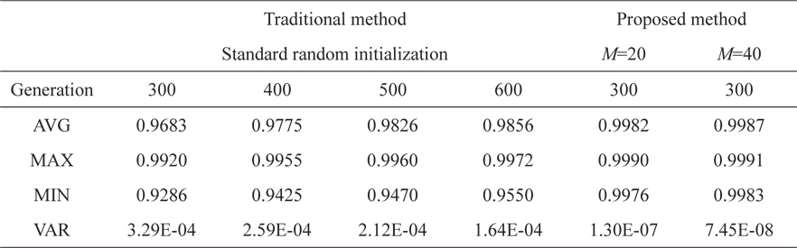
Results for the Hyper Volume Ratio
Next, we investigated the influence of the parameter
By comparing the average and maximum of HVR from Table 3, we observed that the average and maximums value for
On the other hand, if parameter
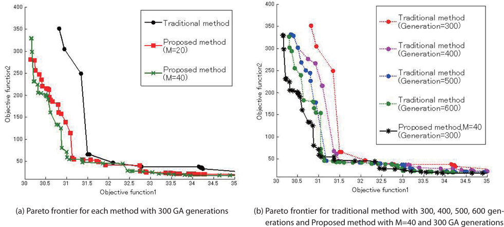
The results of the traditional and proposed methods (
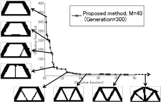
Figure 10 shows the result of the Pareto frontier. In Fig. 10(a), if the traditional and proposed methods have the same computational cost for Step 3, the proposed method with
Figure 11 shows the results for the topology obtained by the proposed method with
Although the proposed method had some additional calculation cost for generating the elite initial population in Steps 1 and 2, we established that the overall computational efficiency of topology optimization using a GA can be greatly improved when compared to the traditional method.
In this study, for efficient multi-objective topology optimization using a GA with bar-system representation, local optimum solutions obtained from the SIMP with weighted sum method were used as an elite initial population for the GA. To verify the efficiency of the proposed method, the traditional method with standard random initialization and the proposed method were compared using the simply supported beam example, and the HVR was calculated to investigate the convergence and diversity of Pareto-optimal solutions. As a result, the proposed method performed better than the traditional method for the average, maximum and variance of HVR measured by Pareto-optimal solutions and the Pareto-frontier, with almost the same computational cost as the traditional method.