Supersonic propulsion systems have applications for a wide variety of aircraft and rockets, operating at flow regimes from subsonic to supersonic. A variety of flow devices for the vehicles operate at a wide range of Mach numbers, so that shock / boundary layer interactions are common, and may have a significant influence on the entire flow field [1-5].
At high Reynolds numbers, flows are very likely to be fully turbulent. With increasing turbulence Mach number, the velocity fields can no longer be assumed to be incompressible. For the transonic and supersonic flow regimes, the shock / boundary layer interaction causes a large increase in turbulence intensity and shear stress. Turbulence modeling for compressible flow has to account for the additional correlations, involving both the fluctuating thermodynamic quantities, and the fluctuating dilatation. To account for the important flow features at transonic and supersonic conditions, the combined models of compressible-dissipation and pressure-dilatation proposed by Sarkar and Wilcox [6-9] were evaluated in this study.
In smooth flow regions with continuous flow variables, the central-differencing schemes based on the Taylor series expansion can be applied, with a certain order of accuracy. In the supersonic regime with discontinuities such as shock waves, however, the scheme becomes numerically unstable. To avoid such non-physical oscillation, the concept of total variation diminishing (TVD) and the AUSMPW+ scheme were used for the inviscid flux calculation, as the upwind schemes [10].
For this study, two-equation turbulence models, low Reynolds k-ε and k-ω SST models, with and without compressible dissipation and pressure-dilatation corrections, are used to evaluate the compressibility effects of turbulent models in transonic and supersonic flows involving flow separation. The four test cases are a 7% arc-bump [11, 12], transonic diffuser [13, 14], the supersonic impinging jet [15], and the supersonic diffuser [16, 17].
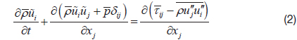
The Favre-averaged governing equations for a compressible flow, based on the conservation of mass, momentum, energy, and species, can be expressed as:
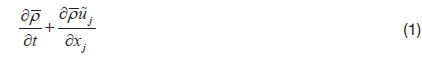

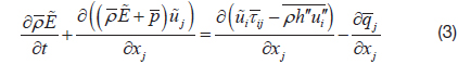
where, superscript “-” represents time averaged quantity, and superscript “~” means mass weighted averaged quantity.
The turbulent models considered for this study are two-equation turbulence models, such as the low-Reynolds number k-ε model, and k-ω SST model.
The standard k-ε model was proposed for high Reynolds number turbulence flows, and is traditionally used with a wall function, and the variable y+ as a damping function. However, universal wall functions do not exist in complex flows, so the damping factor cannot be perfectly applied to the flow with separation. Thus, a low Reynolds number k-ε model was developed, to take account of near-wall turbulence. Shih and Lumley observed that, within certain distances from the wall, all energetic large eddies will reduce to Kolmogorov eddies; and all the important wall parameters, such as friction velocity, viscous length scale, and mean strain rate at the wall, can be characterized by the Kolmogorov micro scale [18].
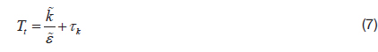
Yang and Shih proposed a time-scale-based k-ε model for the near-wall turbulence, related to the Kolmogorov time scale as its lower bound, so that the equation can be integrated to the wall. The advantages of this model are the lack of a singularity at the wall, and adaptability to separated flow, since the damping function is based on the Reynolds number, instead of y+. The low Reynolds number models have been designed to maintain the high Reynolds number formulation in the log-law region, and further tuned to fit measurements for the viscous and buffer layers [19].
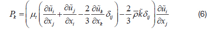
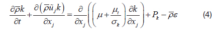
The turbulent kinetic energy and its dissipation rate are calculated from the turbulence transport equations, written as follows:

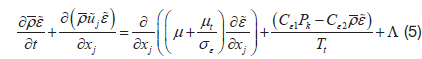
where,


where,
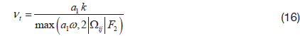
The turbulent viscosity


where,
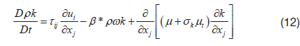
The standard k-ω model predicts the boundary layer near the wall more accurately, but is sensitive to the initial condition of the free flow region. On the other hand, the standard k-ε model predicts the free flow region more accurately, but requires the wall function, and modeling near the wall. Therefore, Menter suggests a blended model, which uses the k-ω model at the inner region of a boundary layer, and then uses the k-ε model for the outer boundary layer, and for free shear layers [20].

For the k-ω SST mode, a blending function, F1, is defined, so as to vary smoothly from a value of 1 near a wall, through the log-law region of the boundary layer, to a value of 0 for the outer wake region of the boundary layer, and for free shear layers. The model coefficients, Φ = {

Two functions are needed; and the eddy viscosity relation for the SST model is given by:

2.3 Compressibility Corrections
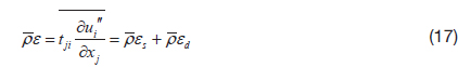
Inspection of the turbulence kinetic energy equation also indicates that the Favre-averaged dissipation rate is given by

where,

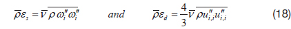
Thus, the compressible turbulence dissipation rate can logically be written in terms of the fluctuating vorticity, and the divergence of the fluctuating velocity. At high Reynolds number, these components are presumably uncorrelated. The quantity
Based on observations from some older Direct Numerical Simulation (DNS), Sarkar et al. [6, 7] postulate that the dilatation dissipation should be a function of the turbulence Mach number,

where, a is the speed of sound. They further argue that the k and ε equations should be replaced by
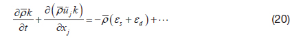
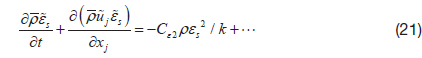
where,

where,

where,
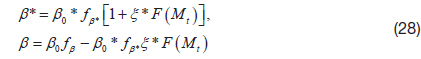
The pressure-dilatation is large, in flows with a large ratio of turbulence-energy production to dissipation. Therefore, Sarkar proposes that the pressure dilatation can be approximated as
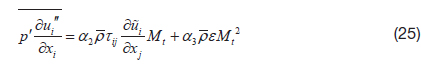
where,

The model has been used for a range of compressibleflow applications, including mixing layers, and attached boundary layers.
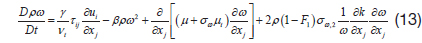
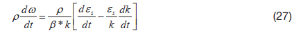
To implement the Sarkar modification in the k-ω model, the formal change of variables given by

Consequently, a compressibility term must appear in the ω equation, as well as in the

where,
The concept of total variation diminishing (TVD), the first of the upwind schemes applied in this study, is that the total variation of any of the physical properties does not increase in time. Temporal discretization is obtained, using a second order dual time stepping integration. The spatial convective terms are discretized with the third-order upwind TVD scheme [6].
In order to avoid such non-physical oscillation, the AUSMPW+ scheme was chosen for the inviscid flux calculation. In previous research, the AUSMPW+ scheme has been known to be more stable, and at the same time less dissipative in supersonic flow, than the Roe scheme. The AUSMPW+ scheme is a modified version of the AUSM (Advection Upstream Splitting Method) family of schemes. The AUSM concept is to use different splitting for the convective fluxes, with each splitting being some function of an intuitively defined interface Mach number. The AUSMPW scheme with pressure-based weight function was introduced to overcome the carbuncle phenomenon, and the overshoot problems behind a strong shock, in the AUSM or AUSMD scheme. The AUSMPW+ scheme is an improved and simplified version of the AUSMPW scheme, with a new numerical speed of sound introduced [21].
The conservation equations for moderate and high Mach number flows are well-coupled, and standard numerical techniques perform adequately. In regions of low Mach number flows, however, the energy and momentum equations are practically decoupled, and the system of conservation equations becomes stiff. To overcome this problem, a two-step dual time-integration procedure designed for all Mach number flows was applied. First, a rescaled pressure term is used in the momentum equation, in order to circumvent the singular behavior of pressure at low Mach numbers. Second, a dual time-stepping integration procedure is established.
The pseudo-time derivative may be chosen, in order to optimize the convergence of the inner iterations, by using an appropriate preconditioning matrix that is tuned to rescale the eigenvalues to render the same order of magnitude, so as to maximize convergence. To unify the conserved flux variables, a pseudo-time derivative of the form Γ
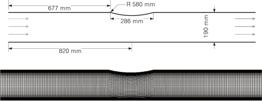
The bump geometry is one of the most broadly used configurations for validating turbulence models in shock / boundary layer interaction in transonic flows. The experiment of Inger and Gendt [11, 12] considers a channel with a flat floor wall, and an upper surface with a bump, which has a circular arc of 580 mm radius of curvature and 20mm height. The inlet flow is subsonic, and there are no incoming standing waves. A schematic of the bump geometry and the computational domain are shown in Fig. 1.
About 29,000 grid points are used; the grid distribution is dense near the wall, in order to accurately capture the boundary layer. The numerical boundary conditions are: stagnation pressure of 140
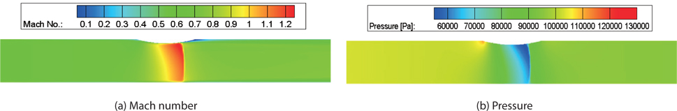
Figure 2 shows the Mach number and pressure contours on the arc bump. The velocity accelerates from transonic (
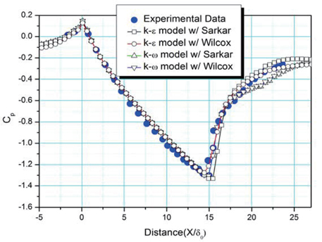
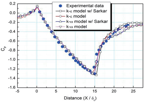
Figure 3 shows the variation of the pressure coefficient
The k-ω SST model predicts most closely the normal shock location, but the pressure recovers slowly after the shockwave. The compressibility effect, the Sarkar model, does not much effect the normal shock location and overall tendency of
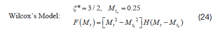
Figure 4 shows a comparison of two different compressibility correction models, the Sarkar and Wilcox models. The Sarkar model considers only the local turbulent Mach number, while the Wilcox model uses both the standard turbulent Mach number, and the local turbulent Mach number, to consider the dilatation dissipation. The result for the low Reynolds k-ε model using the Wilcox compressibility correction model presents better shock location and pressure recovery, than others.
Based on these results, the low Reynolds k-ε model with Wilcox compressibility correction is seen to most accurately predict the experimental data.
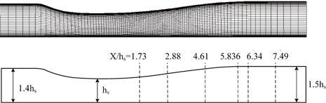
Two-dimensional simulation of the convergent / divergent diffuser described experimentally by Borger [13] has been conducted. The bottom wall of the diffuser is flat, but the upper wall is given by

where,
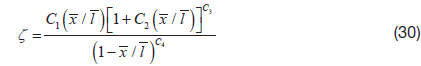
The various constants for the top wall are given in Table 1. The throat height is
[Table 1.] Constants for channel height [15]
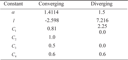
Constants for channel height [15]
Figure 5 shows the geometry and grid distribution of the 100×70 grid points used in this study. At the inflow boundary, the stagnation pressure is 135
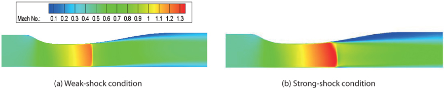
The pressure ratio, defined as the static pressure at the outlet, divided by the inlet total pressure, characterizes the diffuser flow. The weak shock and the strong shock in the diffuser are simulated. The pressure ratios of the weak shock and the strong shock are 0.82 and 0.72, respectively.
Figure 6 shows the flow structure of the diffuser for strong-shock and weak-shock conditions. In the weakshock condition, the normal shock is located at around
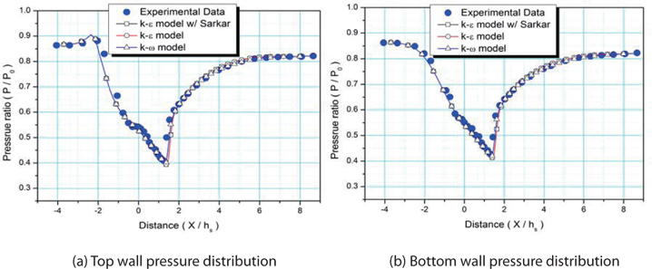
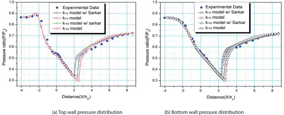
Figure 7 shows a comparison of the pressure ratio along the top and bottom walls of the diffuser, for the weak-shock condition. Both the low Reynolds number k-ε model, and the k-ω SST model, give accurate results. The differences in the results using the Sarkar and Wilcox compressibility models are so small, that the numerical data using the Wilcox compressibility model is not presented.
To investigate the effects of the size of recirculation and shock strength, the strong-shock condition has been investigated. In the strong-shock condition, the separation region is larger, and the shock is much stronger, than in the weak-shock condition. Figure 8 shows a comparison of the pressure ratio for the strong-shock condition. The k-ω SST model predicts the normal shock location better than the low Reynolds k-ε model does. The low Reynolds k-ε model with the Sarkar correction predicts the normal shock location more accurately, but not as well as the k-ω model.
On the bottom wall, the separation region is smaller, than on the top side of the diffuser. The results on the bottom wall behind the normal shock are more accurate, than those on the top wall.
These results show that both two-equation turbulence models have accurate results in the small separation region, but for strong shock condition, the k-ω SST model predicts the shock position better than the low Reynolds k-ε model. The compressibility effects on the k-ω SST model are negligible.
3.3 Supersonic jet impingement
To investigate the compressibility effect, a numerical study of a supersonic jet impinging on an axi-symmetric cone has been conducted.
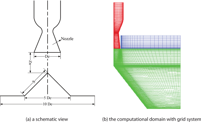
The designed Mach number of the nozzle exit is 2.0, and the mean ratios of nozzle exit pressure to atmospheric pressure (PR) are 1.2 and 2.27. The inlet conditions at PR=1.2 and 2.27 are a total pressure of 921kPa, and 1,742kPa, respectively, and the total temperature is 300K for both cases [15]. The apex angle of the cone is 90˚, and the distance between the nozzle exit and the apex point is Z
Figure 9 (b) shows the axisymmetric computational domain with a grid system. The total number of grid points is about 15,520. Three blocks and six processors are applied, to improve the calculation efficiency.
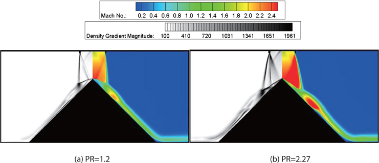
Figure 10 shows the density gradient magnitude, and the Mach number contours. The maximum Mach numbers are about 2.6, in the case of PR=1.2, and about 3.2, in the case of PR=2.27.
The impinging jet flow generates an expansion wave at the nozzle exit, jet boundary, barrel shock, and Mach disk. Due to the impingement on the apex of the cone, the structure of the jet flow becomes more complex. In PR=1.2, the subsonic zone is near the apex of the cone, because the Mach disk is in front of the apex of the cone. The Mach disk rapidly reduces the jet velocity to subsonic. The jet flow through the Mach disk attaches to the surface of the cone, and is recompressed. The pressure recovery at the second compression is more gradual than PR=2.27, as shown in Fig. 10. This means that the degree of the compressibility and the interaction of the shock wave with a turbulent boundary is weaker, than the case of PR=2.27. In PR=2.27, the jet flow core impinges to the apex of the cone, and a stagnation point occurs. The oblique shock at the cone apex closes to the cone wall, and the pressure at the second compression increases more steeply.
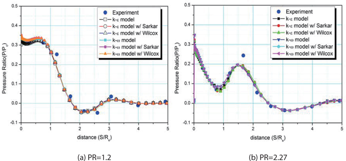
The experimental data and numerical results without compressibility correction are comparable. The compressibility effects are negligible, because 1) the flow separation region at the cone surface is not large, so that the interaction between turbulent boundary and jet flow is not active, and 2) the compressible wave and perturbations due to the impinging on the cone propagate out to the atmosphere, but do not bounce back.
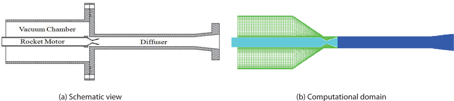
To determine the accuracy of the two turbulence models and the compressibility models in the supersonic regime, the calculation of a supersonic exhaust diffuser configuration was conducted. Fig. 12 shows a schematic view, and the computational domain of the supersonic diffuser.
The dimensions of the model are diffuser length L of 260mm, diffuser diameter D of 21 mm, ratio of length to diameter of diffuser L/D of 12.38, area ratio of diffuser to rocket motor nozzle throat
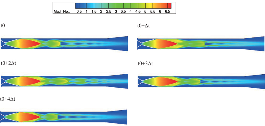
Figure 13 shows the Mach number contours in the supersonic diffuser. The maximum Mach number of about 6.7 appears in the first diamond shock region. A small supersonic pocket occurs at the axis of the diffuser, and moves periodically downstream and upstream. The reason that the shock train accompanying pressure oscillation occurs in the diffuser is that the mass flux and momentum of the exhaust jet are not enough to block the pressure oscillation produced by the acoustic-wave oscillation, in the subsonic region behind the terminal shock. The period of oscillation may relate to the acoustic mode in the subsonic region, after the second shock diamond. Thus, the vacuumchamber pressure stays constant, but the pressure along the wall oscillates periodically, with a certain amplitude, as shown in Fig. 13. If the rocket motor pressure decreases further, the shock train becomes weak.
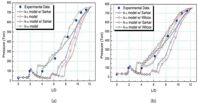
Figure 14 shows a comparison of the pressure along the wall of the diffuser, according to the compressible correction models. The pressure rises behind the impinging point of the jet on the diffuser wall, after the pressure decreases in the expansion region. Afterward, the pressure increases again during the next compression wave; and then it finally rises to atmospheric pressure, at the exit of the diffuser. The results of the k-ω SST model are very different from the experimental data, since the k-ω SST model does not predict the oscillatory flow structure, or the strong unsteady motion. Using the compressibility model, the Sarkar model produces better results, but it does not compare well with the experimental data. The low Reynolds number k-ε model with the Sarkar model is in fairly good agreement with the experimental data. Therefore, in the supersonic regime, the experimental data and the numerical results, from the low Reynolds k-ε model with the Sarkar model, appear to reveal a discrepancy; but the unsteady flow motion in the diffuser is hidden, in the background of the instantaneous data.
Figure 14 (b) shows a comparison of the pressure along the wall, using the Sarkar and Wilcox models. The k-ω SST models are unreliable with both compressibility models, because the k-ω SST model is weak in strong unsteady flow simulation. On the other hand, the low Reynolds number k-ε model has more accurate results, for this particular unsteady flow.
To evaluate numerical modeling of compressibility effects, two two-equation turbulence models, the low Reynolds number k-ε model and the k-ω SST model, with two compressibility models proposed by Sarkar and Wilcox, are applied to simulate four different transonic or supersonic flows. The numerical results are evaluated against experimental data.
For the first validation, a transonic arc bump, the k-ω SST model predicts the normal shock location fairly well, but the pressure after the shock recovers slowly, and the compressibility effects are negligible. The low Reynolds k-ε model with the Wilcox compressibility effect presents better accuracy.
For the second validation case, a transonic diffuser, both the weak shock and strong shock cases are evaluated. Both two-equation turbulence models reasonably predict the flow properties for the weak shock condition, but the k-ω SST model offers more accurate results for the strong shock condition. The compressibility effects on the k-ω SST model are negligible.
For the third validation case, a supersonic impinging jet, supersonic jets of pressure ratio (PR) 1.2 and 2.27 are investigated. Both two-equation turbulence models have similar wall pressures, with reasonable accuracy against experimental data, because the flow separation size is small, and the compressible wave and perturbation due to the impinging on the cone smear out to the atmosphere.
Finally, an unsteady supersonic diffuser was evaluated for the test of the compressibility correction models. The low Reynolds k-ε equation with Wilcox compressibility model provides the most accurate results for this particular unsteady flow.
In summary, compressibility effects on the turbulence model are very important in supersonic flow with large flow separation, because of the strong interaction between shock and boundary layer. The compressibility correction model has a stronger influence on the k-ε model, than on the k-ω SST model.


![Schematic of the geometry, and a magnified view of the representative meshing around the transonic bump [12]](http://oak.go.kr/repository/journal/13485/HGJHC0_2013_v14n4_387_f001.jpg)


![Constants for channel height [15]](http://oak.go.kr/repository/journal/13485/HGJHC0_2013_v14n4_387_t001.jpg)
![Schematic of the geometry, and grid distribution of the transonic diffuser [14].](http://oak.go.kr/repository/journal/13485/HGJHC0_2013_v14n4_387_f005.jpg)

![Schematics and computational domain of the supersonic nozzle and axi-symmetric cone [15]](http://oak.go.kr/repository/journal/13485/HGJHC0_2013_v14n4_387_f009.jpg)