This study examined the dependency of hot carrier degradation on the time exponent n, as a function of the stress time, as well as the influence of hot carrier degradation on lifetime projections by data interpolation and extrapolation, which are used to evaluate process qualification and reliability. The discrepancy in the n value given by extrapolative data analysis can result in erroneous hot carrier injection lifetime projections, despite the reliable and mature front-end-of-line process. Because the n value is dependent on the changes in the saturation drain current (IDSAT), interpolative data analysis gave more reliable lifetime projections than the extrapolative data analysis, without extending the stress time. Failure time obtained by interpolation was different from that by extrapolation because the time exponent, n, changes with the variation rate of IDSAT. The errors of the parameter, m, in the HCI model were attributed to the difference in failure time, which in turn affected the lifetime projections. A modified method was suggested to minimize the errors in lifetime projections with the conventional stress time frame. A lower rate of change of IDSAT, which allows interpolation, was applied as the failure criterion instead of the actual failure criterion of the device to extract a more accurate value for the parameter, m, with the results, because the parameter, m, is an important factor of a lifetime projection at a given level. The use of this lower variation rate of IDSAT as the failure criterion eliminates the need to account for the changes in failure criteria. This method estimated lifetime projections more reliably.
Semiconductor manufacturing technology has driven the associated metal oxide semiconductor field effect transistor (MOSFET) scales close to their physical limits for faster and larger integration. Hot Carrier Injection(HCI) is one of the major factors affecting device reliability which has limited device scaling over the last few decades[1-4]. A high lateral electric field supplies sufficient energy to electrons in the pinch-off region to overcome the potential barrier under HCI, which degrades the current-voltage characteristics by damaging the drain side [5]. The process-conditions-dependent HCI characteristics and HCI mechanisms were investigated by HCI modeling to predict the level of HCI-induced device degradation [6-10]. HCI-induced device degradation under circuit operation has been predicted by using several empirical and semi-empirical models, but even the more complicated modeling processes have provided, little insight into the physical mechanisms of the degradation in short-channel devices. Therefore, HCI-induced device degradation requires more reliable modeling. Competitive and reliable evaluations require a demonstration of the optimal trade-off between reliability and speed [11]. The extraction of accurate modeling parameters is important as much as the determination of an appropriate modeling method, whereas acceleration testing has been carried out for a lifetime projection. In this study, the dependence of the hot carrier time exponent on the stress time as well as its influence on the lifetime projection was examined experimentally to estimate HCI-induced device degradation, competitively and reliably.
The following describes the general HCI acceleration testing process [12]:
(A) determine the worst-case biasing configuration
(B) stress the device and characterize it at various stress intervals
(C) plot the delta shift data
(D) determine the failure criteria
(E) calculate the failure time(tFAIL) for each stress using

where ΔIDSAT is the rate of the changes in drain current in the saturation mode, t is the accumulated stress time, and A and n are fitting parameters.
(F) repeat steps(B)-(E) for various drain voltage(VD) stresses,
(G) plot tFAIL for each stress voltage and (H) perform linear regression to extract H and m using
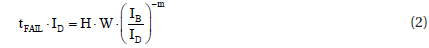
where tFAIL is the failure time, which means the HCI lifetime of the device, W is the width of a transistor, ID and IB are drain current and substrate current in stress, respectively, and H and m are the fitting parameters.
(I) determine IB and ID at the operating condition(IBOP and IDOP)
(J) calculate tFAIL at IBOP/IDOP.
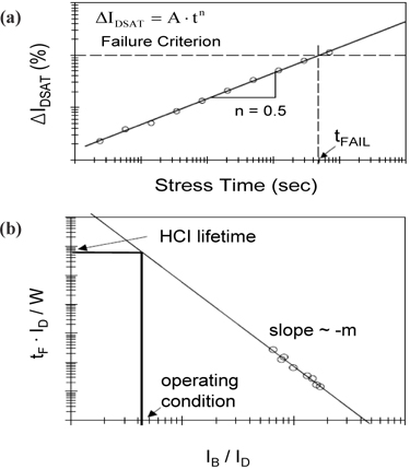
Equation (1) can be used to determine the failure time (tFAIL) in step (E) in the above process, as shown in Figure 1(a), and either interpolation or extrapolation is applied in this case. If the data obtained from the test are above the failure criteria specified in step (D), the failure time can be determined by interpolation. On the other hand, if the resulting data obtained from the testing are not above the failure criteria, failure time can be determined by extrapolation. In this case, the obtained failure time can be less accurate than that determined by interpolation. The device lifetime can be obtained from a plot of the failure times obtained in step (E), as shown in Fig. 1(b), by applying equation(2). The parameter, m, is important for calculating device lifetime. That is, it is necessary to accurately calculate m to obtain a calculated lifetime with a small error. In this paper, the changes in the time exponent, n, resulting from the stress time and failure time errors were examined. In addition, the effects of failure time errors on the parameter, m, and device lifetime were also examined. A novel lifetime projection that reduces such an effect was attempted for accurate device lifetime prediction.
The samples used in this study were introduced by 110-nm technology. The gate oxide was grown to a thickness of 6.2 nm (equivalent oxide thickness, EOT) by thermal oxidation. A n-channel MOSFET with a lightly doped drain (LDD) structure was fabricated with a nominal gate length and width of 0.64 and 10 μm, respectively. Drain voltages (VD) of 5.3, 5.5, 5.8 and 6.1 V were applied to the packaged samples to examine the characteristics of the hot carrier. At each drain voltage, a gate voltage (VG) was applied until the substrate current (IB) reached the maximum (source and substrate were grounded). Stress was imposed for a maximum of 2,300,000 seconds, and was interrupted periodically to measure the drain current in the saturation mode. The saturation drain current (IDSAT) was measured at VDD = 4.3 V, and the rate of change of IDSAT was set to 10% as the failure criteria. All studies were carried out at room temperature.
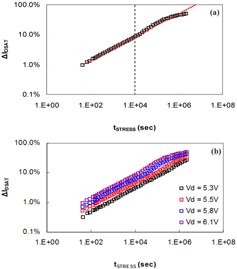
HCI degradation is characterized by a power-law with a dependence on the stress time, as shown in equation (1), where the time exponent, n, was approximately 0.5 [12,13]. Figure 2(a) shows the rate of change of IDSAT with increasing stress time at VD = 6.1 V as the induced stress. The data obtained for 10,000 seconds were used to plot the power-law trend curve (the red solid line in Fig. 2(a)). The data after 10,000 seconds deviated from the trend curve. A larger rate of change than that of the trend curve was observed after 10,000 seconds, and the rate of change saturated after a certain time. In this case, an accurate prediction could not be made for the data after 10,000 seconds by using the data obtained before 10,000 seconds. According to Aono [14], the time exponent of the negative bias temperature instability (NBTI) differed according to the stress time, and the same time exponent was shown for the same stress time, regardless of the stress voltages. HCI showed the same trend for four VD stress conditions, as shown in Fig. 2(b).
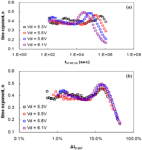
Figure 3(a) shows the rate of change of IDSAT with increasing stress time for each stress condition. The result for 6.1V showed a similar trend to those of the remaining 3 conditions. Figure 3(a) also shows the time exponent, n, according to stress time. Different time exponents were exhibited in the same stress time zone depending on the stress condition, unlike the NBTI. The same time exponent, n, was observed at the same rate of change of IDSAT, as shown in Fig. 3(b), which was re-plotted based on the rate of change of IDSAT in Fig. 3(a). This is because the recovery is relatively high after interrupting the stress to measure the device parameters for NBTI. Therefore, the changes in the time exponent, n, are dominated more by the stress time than by the changes in the device parameter. Accordingly, there is no significant recovery in the HCI, which means it is affected by the changes in the device parameter [13,15].
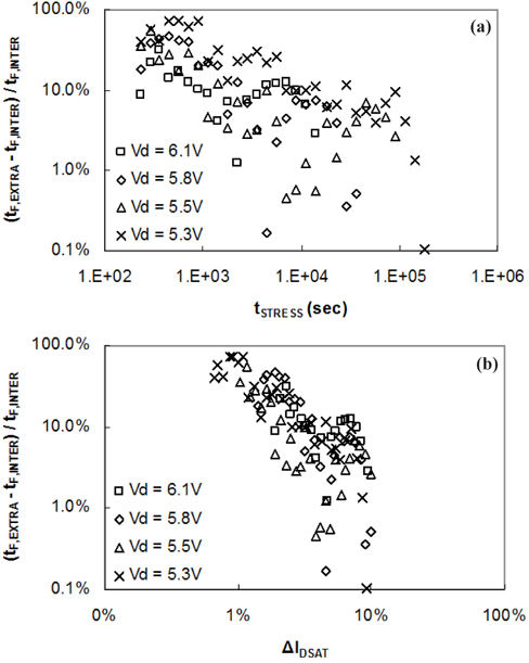
In developing the process, the wafer level reliability (WLR) was evaluated at high acceleration for faster feedback, and the lifetime obtained from the evaluation of the WLR contained some uncertainty due to the high acceleration. Such an evaluation of the WLR is normally carried out for a stress time of 10 to 105 seconds [16]. If the data obtained from the evaluation change above the specified failure criteria, the failure time is determined by interpolation(tF,INTER), otherwise by extrapolation(tF,EXTRA) if the changes are smaller than the failure criteria. Because it is generally impossible to have sufficient stress time for an evaluation due to the limited time and equipment, extrapolation rather than interpolation is applied. The failure time determined by extrapolation shows some differences from the actual failure time (tF,INTER) because the time exponent, n, changes depending on the rate of change of IDSAT. Accordingly, the device lifetime finally obtained contains errors. Figure 4(a) shows the differences in the failure time as (tF,EXTRA - tF,INTER) / tF,INTER for different stress times. A shorter stress time results in larger differences in the failure time, regardless of the stress conditions. As for the rate of change of IDSAT, the smaller the rate of change of IDSAT with respect to the failure criteria results in greater errors in the failure time, as shown in Figure 4(b). If the time exponent, n, depends on the rate of change of IDSAT and the failure time is obtained by extrapolation, failure time will be different from that obtained by interpolation.
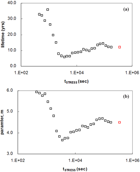
Figure 5(a) shows the device lifetime according to the applied stress time. The lifetime shown by a red square was obtained with the failure time determined by interpolation. The lifetime decreases at the shorter stress times, but increases sharply at the longer stress times. Errors in lifetime are encountered because the failure time is determined by extrapolation at the shorter stress times. The difference between the predicted and the actual device lifetime is in the range of 50% to 200%. The lifetime changes in proportion to the parameter, m, due to a change in the parameter, m, of equation (2), as shown in Fig. 5(b). The parameter, m, changes with the stress time because the calculated failure time is affected by changes in the time exponent, n, whereas the failure time is determined by extrapolation. The changes in the time exponent, n, are divided into 3 sections: The first section shows a gradually decreasing time exponent, n. The second section shows an increasing time exponent, n. The third section, on the other hand, shows a decreasing time exponent, n. An increasing or decreasing failure time depends on the section used for the extrapolation.
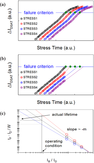
Figure 6 shows the changes in the parameter, m, according to stress time. Figure 6(a) shows the rate of change of IDSAT for four stress conditions, in which the evaluation continues above the failure criteria to calculate the failure time under each stress condition by interpolation. The calculated failure times are shown by green circles. Figure 6(b) shows smaller rates of change of IDSAT than the failure criteria, which includes the power-law trend line obtained with the last three datasets under each stress condition, in which the points where the trend line meets the failure criteria are the failure times (extrapolation). Four green circles are the failure times determined by interpolation in Fig. 6(a). For stress 1, the rate of changes of IDSAT reached the failure criteria, in which the time exponent, n, was approximately 0.46. For stress 2, the failure time determined by interpolation was shorter than the failure time estimated by extrapolation. A shorter failure time was obtained when extrapolation was applied because the time exponent, n, of stress 2 was 0.51, which is greater than that of stress 1 (0.46). When the time exponent, n, of stresses 3 and 4 were 0.37 and 0.35, respectively, which were smaller than that of stress 1 (0.46), a longer failure time was obtained by extrapolation. If a shorter failure time than the real failure time was obtained, as in the stress 2 condition, the parameter, m, of equation (2) would be smaller, whereas the longer failure times in stresses 3 and 4 resulted in a larger parameter, m, as shown in Fig. 6(c). That is, the difference in the time exponent, n, of the data used to determine the failure time caused the changes in the calculated failure time, and the different calculated failure times affected the parameter, m, and the calculated lifetime.
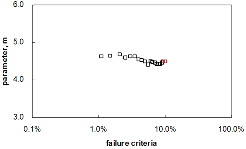
The factors that affect the device lifetime estimation by extrapolation are not only the changes in failure time according to the time exponent, n, but also the errors of the parameter, m, due to the difference in failure time. First, the parameter, m, which affects the estimation of the lifetime, was examined to reduce the errors in the lifetime estimated by extrapolation. Figure 7 shows the parameter, m, according to the failure criteria, the parameter values of 1.8 to 4.1% were more stable than those of 18.6 to 31.9% according to stress time in Fig. 5(b). Therefore, more stable values can be obtained if interpolation is used instead of extrapolation to determine the failure time to calculate the parameter, m. The general HCI acceleration testing process, as described in introduction, was modified based on this result. Criteria 2 is specified in step (D) to be used in finding the parameter, m, with the failure criteria (criteria 1) of the device. Criteria 2 should be low enough to allow an interpolation under all stress conditions. In step (E), failure times 1 and 2 were identified under each stress condition using criteria 1 and 2 specified in step (D). Step (H) is comprised of 2 sub-steps: first, parameter, m, is obtained using failure time 2, which was identified by applying criteria 2, and second, the parameter, H, is then calculated using parameter, m, with failure time 1 under the stress condition with the greatest changes in IDSAT. Failure time 1 was used under the stress condition with the largest change in IDSAT because there are larger errors in the failure time as the difference between the changes in IDSAT and failure criteria increase, as shown in Figure 4(b). The modified testing process was applied to predict the actual HCI lifetime. The result was compared with the result of the conventional testing process shown in Table 1. In the case of a stress time of 360,000 seconds, the rate of change of IDSAT was at least 10% under all conditions, and the lifetime was obtained by interpolation after applying criteria 1 (based on 10% change of IDSAT). In the case of a stress time of 90,000 seconds, the rate of change of IDSAT was less than 10%. The lifetime, which was identified with the parameter, m, obtained by interpolation using criteria 2, was 11.17 years with a smaller error than that of the actual device lifetime obtained by the conventional scheme (lifetime = 14.36 years with an error of 20.1%). For the other stress times, the two schemes were compared. The errors of the conventional scheme, ranged from 52.0 to 20.1%, but those of modified scheme ranged from 22.7 to 14.8%, so the modified scheme allows a more accurate estimation of the lifetime.
[Table 1.] Comparison of the lifetime between the two schemes.
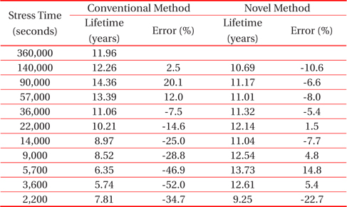
Comparison of the lifetime between the two schemes.
The effect of the HCI stress time on the time exponent, n, and on the lifetime projection was examined. Unlike NBTI, in which the time exponent, n, is mostly affected by the stress time rather than the device parameters, the HCI time exponent, n, changed with the rate of change of IDSAT. The failure time obtained by interpolation was different from that obtained by extrapolation because the time exponent, n, changed with the rate of change of IDSAT. The errors of parameter, m, in the HCI model were attributed to the difference in the failure time; these errors, in turn affected the lifetime projection. For an accurate lifetime projection, a modified method was suggested to minimize the errors in the lifetime projection under the conventional stress time frame. A lower rate of change of IDSAT, which allows interpolation, was applied as the failure criteria instead of the actual failure criteria of the device to extract a more accurate parameter, m, with the results, because the parameter, m, as an important factor for a lifetime projection at a given level without needing to take the changes in failure criteria into account. This method estimate the lifetime projection more reliably with errors of 22.7 to 14.8% than the conventional methods, which had errors of 52.0 to 20.1%.


![(a) Device degradation plot in HCI stress [10]. Use equation (1) to calculate the HCI failure time. For the failure criteria, ΔIDSAT of 10% was applied and the failure time was calculated by interpolation, (b) example of a calculation of the HCI lifetime [8]. The open circles represent the failure times under the stress conditions, and the gradient of the straight lines in the log-log scale plot is the parameter, m, of equation (2).](http://oak.go.kr/repository/journal/13465/E1TEAO_2014_v15n3_130_f001.jpg)