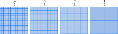
A major advantage of wavefront reconstruction based on a series of diffracted intensity images using only single-beam illumination is the simplicity of setup. Here we propose a fast-converging algorithm for wavefront calculation using single-beam illumination. The captured intensity images are resampled to a series of intensity images, ranging from highest to lowest resampling; each resampled image has half the number of pixels as the previous one. Phase calculation at a lower resolution is used as the initial solution phase at a higher resolution. This corresponds to separately calculating the phase for the lower- and higher-frequency components. Iterations on the low-frequency components do not need to be performed on the higher-frequency components, thus making the convergence of the phase retrieval faster than with the conventional method. The principle is verified by both simulation and optical experiments.
Optical wavefronts that are reflected by or transmitted through an object experience amplitude and phase modulation by the object. If the light field is passing through an object, the measured wavefronts carry information related to the phase delay caused by the object, which is due to the refractive index and shape of the object; thus when the wavefront is measured, the thickness and shape of the object can be obtained. If the light field is reflected by an object, the wavefront carries information regarding the topology of the object, and thus can be used to measure the surface profile of the object. Hence wavefront measurements can be utilized in many areas, including imaging, surface profiling, adaptive optics, astronomy, ophthalmology, microscopy, and atomic physics [1, 2]. However it is not possible to detect the phase using modern detectors because the oscillation frequency of light is too high to be followed by detectors. Therefore, many attempts to acquire phase information have been made in the past. The techniques for this can mainly be categorized into two types, one based on interferometry and the other a phase-retrieval method based on capturing the intensity of the object beam. The interferometry method, generally referred to as holography, records the interference pattern of an object beam and a reference beam. This process converts phase information to intensity modulation [3]. However, introducing a reference beam requires a complicated interference experimental setup, which also induces some other problems in hologram reconstruction, such as the DC-term problem and the twin-image problem. These problems require a more complicated experiment setup [4, 5].
Wavefront reconstruction using phase-retrieval techniques does not require any reference beam. Generally, several diffracted intensity images and some digital image post-processing are needed. Deterministic phase retrieval using the transport of intensity equation (TIE) works under conditions of the paraxial approximation, which limits its application in general [6-8]. Iterative phase-retrieval methods mainly involve the use of the Gerchberg-Saxton (GS) and Yang-Gu (YG) algorithms, which use prior knowledge of the object as constraints [9-11]. For the case of an object with an unknown constraint, it is difficult to reconstruct the wavefront using the GS and YG algorithms. Various approaches have been proposed to solve this problem. One approach is to characterize the object indirectly, using an aperture to capture small images and then obtain the object constraint [12], or using a known illumination pattern as a constraint instead of the object constraint [13]. The other approach is to use two or more intensity images with variations, which can be produced by capturing intensity images with different focuses [14-16], translating an aperture transversely [17], or shifting the illumination [18]. However, all of these approaches require additional optical components and involve complicated digital postprocessing.
Pedrini
It is known that the number of captured images affects reconstruction quality, with more intensity images resulting in higher-quality reconstructions [23]. However, capturing more intensity images requires more movement steps of the camera or the object, which makes the captured images sensitive to small misalignments in the experimental setup, and thus the noise in the captured intensity images becomes more serious. Furthermore, capturing more intensity images requires more experimental time, which makes the method not suitable for dynamic-object or real-time applications. In order to improve the capabilities of SBMR [19], beam splitters [24], spatial light modulators (SLM) [25, 26], or deformable mirrors (DM) [27] were used to achieve single-shot or single-plane intensity image capturing processes. However, beam splitters cause the attenuation of illuminating light. In the cases of SLM and DM, the simplicity of the experimental setup is sacrificed. A random amplitude mask [28] and random phase plate [29] have also been used to transform low frequency components to fast varying high frequencies, which requires fewer iterations for reconstruction. However, an amplitude mask results in the diminution of light energy, and the use of a phase plate requires difficult fabrication.
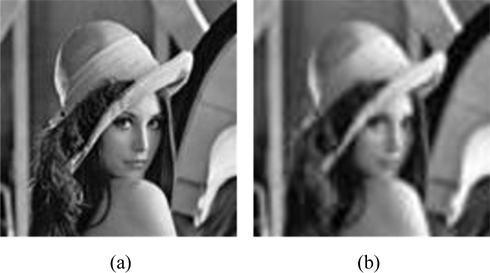
Multiscale signal representation is a very efficient tool that can be used in signal and image processing [30, 31]. It represents signals or images with different resolutions: The high-resolution images carry the high spatial frequencies of the original image, and the low-resolution images carry the low spatial frequencies. An example is shown in Fig. 2. Figure 2(a) shows an image with 128 pixels and Fig. 2(b) shows a scaled image with 64 pixels, which looks like a low-pass-filtered image of Fig. 2(a), i.e. Fig. 2(b) contains the low frequencies of the image [32]. In the conventional phase-retrieval method, because the high-frequency components of the object vary faster than the low-frequency components, the variation between two diffracted intensity images is larger for the higher-frequency components of the object than the low-frequency components of the object. Therefore, fewer iterations are needed to recover the high-frequency than the low-frequency components. This is why the convergence proceeds rapidly in the beginning, and then becomes very slow.
In this study, we optimized the SBMR method by using a multi-scale technique. The captured diffractive intensity images are resampled to several images with different resolutions. Phase retrieval is first performed on the images resampled with a lower resolution, and then transferred to images that are resampled with a higher resolution. This corresponds to performing more iterations for the low-frequency components than the high-frequency components. Suppose a captured image is resampled to some number
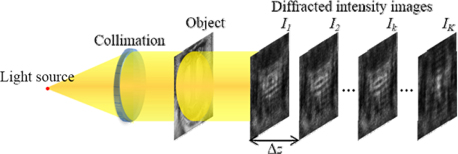
In our proposed algorithm the capturing process is the same as that for the conventional method, as shown in Fig. 1. A series of speckle diffractive intensity images
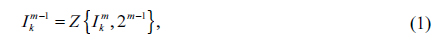
where
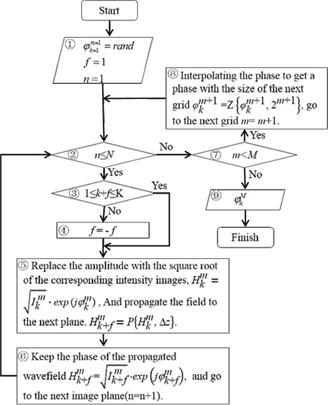
Figure 4 shows the flowchart for our proposed algorithm. The circled numbers in this figure denote the steps of the procedure. In the flowchart,
The details of the iterative procedure are as follows.
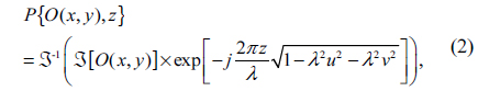
Step 1: Set the initial value. The procedure starts from the first image at the first level, i.e. k=1 and m=1. The initial complex field is a composite of an amplitude and a random initial phase. The square root of the intensity is used as the amplitude, and the initial phase is a random distribution that has 21 pixels, which is the size of the lowest sampled level. Step 2: Check the current iteration number. When the iteration number reaches the maximum iteration value, go to the next level, i.e. go to step 7; otherwise, perform an iteration at the current level, i.e. go to step 3. Step 3: Decide which process should be continued according to whether the current image is the last, the first, or not in the current group. If not, do the forward propagation to the next image, i.e. go to step 5; otherwise, do the backward propagation, i.e. go to step 4. Step 4: Reverse the propagation direction. Step 5: Build the complex wave field. Use the square root of the current intensity distribution as the amplitude, and the previously calculated phase as the phase: Then propagate this wavefield to the next plane: Here P indicates the angular spectrum propagation of the Rayleigh-Sommerfeld diffraction [40]:

where J is the operation of the Fourier transform, λ is the illumination wavelength, and (u, v) are the coordinates after propagation.Step 6: Updating the amplitude of the calculated complex wavefront in the next plane by using the square root of the intensity image at this plane: Also update the index of the iteration and intensity image. Shift the process to the next image plane, i.e. go to step 2. Step 7: If the current level is the last level, retain the calculated phase in step 6 as the final solution. Otherwise, using the solution in step 6 as the initial phase of the next level, go to step 8. Step 8: Interpolate the calculated phase in step 6 to the size of the next level using Eq. (1). Here the second parameter in this equation should be 2m+1. Perform steps 2 to step 8 until the iteration number that was set previously is reached.
From the final calculated wave field, the wavefront at all the captured image planes can be obtained by propagating this field, and the object can be reconstructed by back-propagating the wavefront to any image plane.
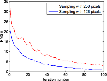
As presented in the introduction, the images sampled with fewer points carry the low-frequency components of the image, which requires fewer iterations in the phase reconstruction, and vice versa. This is indicated in Fig. 5. The two images with 128 and 64 pixels in Figs. 2(a) and 2(b) are reconstructed using the conventional error-reduction method. The normalized root-mean-square errors (RMSEs) according to the iteration number are plotted. The red dashed and blue solid lines indicate the convergence of the iterations for Figs. 2(a) and 2(b), respectively. It can be seen that the iterative convergence for the image sampled with 64 pixels is faster than for that with 128 sampling points.
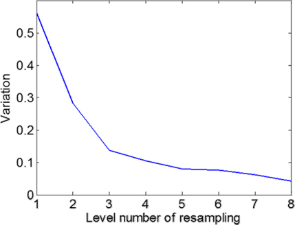
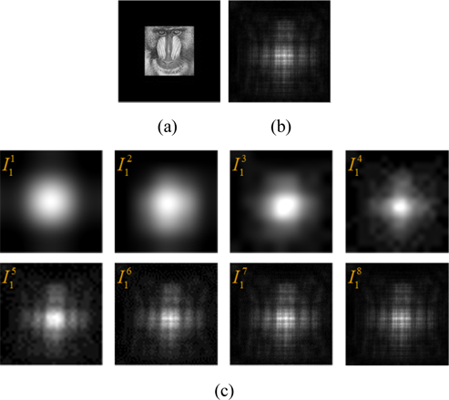
Resampling the images also produces increased variations between images. Figure 6 shows an example of the variations between diffracted images along the optical axis with varying resampling levels. Figure 2(a) is used to generate two diffracted images with a slice-depth difference. The two images are resampled to 8 levels respectively. The variations for different level images are then calculated. The horizontal axis represents the level number and the vertical axis represents the variations with the corresponding sampling level on the horizontal axis. This figure demonstrates that the variation between images at two planes along the optical axis increases with decreasing sampling numbers, which is the requirement for achieving fast convergence in iterative phase-retrieval techniques. This can be attributed to the fast convergence of phase retrieval because the amount of defocusing between the diffracted intensity images affects the accuracy of the phase retrieval [41]. The amount of defocusing can be obtained with a larger depth difference, in our method, by just carrying out a post-resampling of the diffracted images.
Based on the two points presented above, we can speculate that resampling diffracted intensity images with different levels makes it possible to perform a faster-converging iterative phase retrieval.
In the simulation, the object is a composition of the amplitude pattern shown in Fig. 7(a) and a random phase distribution ranging from 0 to 2π. The size of the object is 256×256 pixels. The object is padded with zeroes to avoid energy leakage from the edges of the captured intensity images. In experiment, this corresponds to making almost all of the intensity distribution be within the camera sensor area. The object is illuminated by a light source with a wavelength of 532 nm. Five intensity images are captured by a CCD camera with a pixel pitch of 4.65 μm. The nearest capture plane is located at a distance from the object plane of
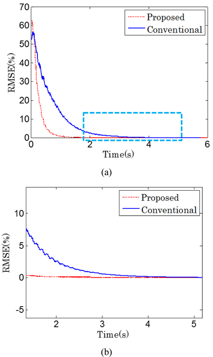
The original image is reconstructed by both the conventional and the proposed methods, respectively. The normalized RMSE is used to measure the results. Figure 8 shows the RMSE with respect to time consumption. The proposed and conventional reconstructions are plotted as a red dashed line and a blue solid line, respectively. Figure 8(b) is the square area crossed by the blue dashed line in Fig. 8(a). From Fig. 8(b) it can be seen that the conventional method reached a minimum RMSE value at about 4.5 seconds, while the proposed method arrived at the same RMSE value in about 2.2 seconds, which is about 51% faster than the conventional method.
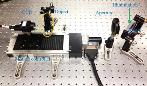
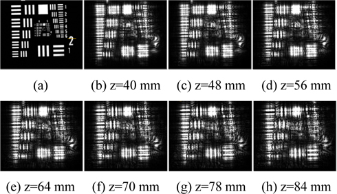
In the experiment, a laser with a wavelength of 532 nm was used to illuminate a Newport USAF 1951 resolution chart. In the resolution chart the background area is opaque, while the line area is transparent. The light wave after the object is modulated in the line area and stopped in the opaque area. Thus the optical wavefront, just after the object, reflects the shape of the resolution chart. By reconstructing the wavefront at the location of the object, the shape image of the object can be reconstructed. Seven diffracted intensity images were captured by a Point Grey FL2-14S3M/C CCD camera. The first image was located a distance of 40 mm from the target, and the interval between the two images was 8 mm. Figure 9 shows the experimental setup. Figure 10(a) shows the directly captured image of the resolution chart, while Figs. 10(b)-(h) show the captured diffracted intensity images. The wavefront at the first plane was calculated by both the conventional and the proposed methods, respectively. The object was reconstructed by digitally propagating the calculated wavefront.
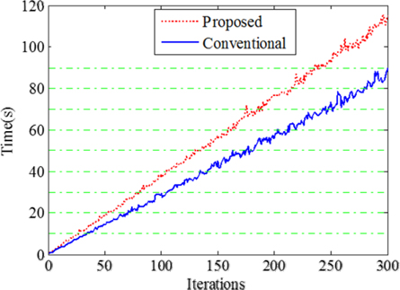
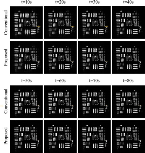
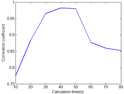
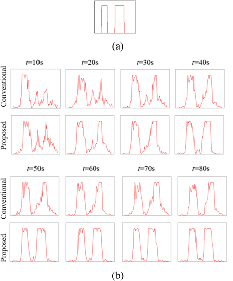
Three hundred iterations were performed in both the conventional and proposed methods. The corresponding time consumption is shown in Fig. 11. The horizontal dashed lines are the chosen timelines for convergence comparison. The red dashed line and blue solid line represent the proposed and conventional methods, respectively. The horizontal axis values of the two intersection points on each horizontal dashed line indicate the numbers of iterations used in the conventional and proposed methods, respectively, and are listed in Table 1. The corresponding reconstructed images for the iteration numbers in Table 1 are shown in Fig. 12. The lines crossing the “2” character are plotted in Fig. 13(b). Figure 13(a) shows a plot corresponding to the directly captured object, i.e. Fig. 10(a), which is used as the reference. From Fig. 13 it can be seen that, in the conventional method, about 80 seconds were needed to obtain the best reconstruction. In order to find how much time is needed for the proposed method to reconstruct the image with a quality similar to this image, we compared this image with the proposed reconstructed images for time consumptions of 10s, 20s, 30s, 40s, 50s, 60s, 70s, and 80s. The correlation coefficients are plotted as Fig. 14. From this figure, a similar image was obtained with the proposed method within 40 seconds. This means that the proposed method is capable of obtaining a similar reconstruction to the original with a time consumption of about 40 seconds, which is about 50% faster than the conventional method with the case of our example images. This result is also in agreement with the simulated results. The small stagnation in the reconstructions by the proposed method is induced by the noise in the experimental images.
[TABLE 1.] Iteration requirements for the crossed points in Fig. 11
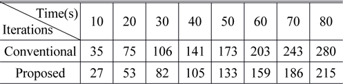
Iteration requirements for the crossed points in Fig. 11
We propose a fast-convergening wavefront reconstruction algorithm by resampling diffractive intensity images. Both simulation and experimental results show that the convergence of the proposed method is about 50% faster than the conventional method for the case of our test images. We expect that the proposed method can be applied to real-time phase-retrieval applications, with further development of computer processor speeds.