검색 전체 메뉴
PDF
맨 위로
OA 학술지
Adaptable Center Detection of a Laser Line with a Normalization Approach using Hessian-matrix Eigenvalues
  • 비영리 CC BY-NC
  • 비영리 CC BY-NC
ABSTRACT
Adaptable Center Detection of a Laser Line with a Normalization Approach using Hessian-matrix Eigenvalues
KEYWORD
Laser line , Center detection , Normalization approach
  • I. INTRODUCTION

    Vision measurement of structured light is one of the important approaches for three-dimensional object measurement and has the advantages of bring noncontact and informative, with moderate measurement speed and measurement accuracy [1]. It is widely used in the inspection of automobile parts, the morphology testing of vehicle surfaces, medical CAD/CAM, quality assurance, and other metrology fields [2-6]. A measurement system for structured light generally consists of a camera, a laser projector, and a computer [7, 8]. The image from a laser line shining on the object is the source of information to achieve the measurement task. One of the key steps in the whole measurement task is to extract accurately the center positions of a laser line [9, 10]. The ideal center positions of a laser line should be a single-pixel-wide curve located in the center of the light line [11, 12]. As an actual light plane is produced with a certain thickness, the intersection curve of the light plane and measured object surface also has a certain width. Therefore, fast and accurate center extraction of a laser line in a test image is of great significance to the vision measurement system of structured light [13, 14].

    Currently, extraction methods for the centers of a laser line can be classified into two categories. One category is based on pixel level, such as the extreme-value method [15, 16], threshold method [17-19], and directional-template method [20-22]; the other category is executed at the subpixel level, including the gray-centroid method [23, 24], curve fitting [25, 26], and the Hessian-matrix method [27-29].

    The principle of the extreme-value method [15, 16] is to choose the pixel with maximum gray value on the transverse section of a laser line as the center of the laser line. This method achieves simple and fast extraction and gives better recognition results when the grayscale distribution of a light line obeys an ideal Gaussian distribution. Nonetheless, it is susceptible to noise. Noisy points in an image captured by a camera often remain in the image even after filtering. Therefore, in the actual measurement, when the grayscale distribution of a laser line is not strictly in accordance with a Gaussian distribution or is affected by noise, the recognized centers will deviate from the actual centers of laser line, leading to extraction results with lower accuracy. The threshold method [17-19] sets a boundary threshold to obtain two borders in the transverse section of a laser line, and the centers of the laser line are regarded as the centers of the two borders. The characteristics of this method are similar to those of the extreme-value method, which allows high processing speed. However, recognition errors are brought about when the grayscales of the transverse section in a laser line are distributed asymmetrically or affected by noise. In addition, it is also a complex issue to select a reasonable threshold. Useful pixels are missed if the threshold is too high, while useless pixels are generated if the threshold is too low. As the threshold interferes with the results of this method, the threshold method is often used with other methods as the first step to select the centers of the laser line. The directional-template method [20-22] sequentially convolutes the 0°, 90°, and 45° directional templates with the image containing a laser line. By this method, extreme points in the transverse section of the laser line are strengthened after convolution, while the other surrounding points are suppressed correspondingly. If the direction of the laser line is identical to the template orientation, the locations of the extreme points will be more prominent. Comparing the process results of each directional template, the point with maximum value is the section center of the laser line. The directional-template method improves the former approaches by repairing disconnected lines and noise suppression. However, this method increases the amount of computation and data storage needed, since each line in the image should be convoluted with the templates in four directions. Overall, the methods above extract the centers of the laser line at the one-pixel level of precision. To enhance the measurement accuracy of the structured light method, researchers further proposed several extraction methods at the sub-pixel level. The gray-centroid method [23, 24] directly calculates the grayscale center along the abscissa as the center position according to the arrangement of gray values of a laser line in a certain range. First, the maximum grayscale point of the laser line is found by the extreme-value method above; then several pixels are chosen around this maximum point. The center position of the laser line in this region is determined by the centroid equation. The gray-centroid method investigates the light intensities of all the points around the extreme point, avoiding the negative impacts of uneven light distribution on the extraction results. Nevertheless, as this method searches for the maximum grayscale point of the laser line by applying the extreme-value method, it is also very sensitive to noises, as is the extreme-value method. Since the gray-centroid method performs line scanning, the extraction accuracy is affected by the curvature of the laser line, so this method is generally used for a laser line with little curvature. The curve-fitting method [25, 26] outlines the grayscale distribution of a transverse section of a laser line employing a Gaussian curve or a parabola. The center point of the transverse section is the local maximum of the fitted curve. This method is only valid for a wide laser line with constant direction of its normal vectors. Additionally, the actual grayscale distribution of pixels in a laser line is not strictly symmetrical, so the extreme point found via the curve-fitting process often deviates from the actual center of the laser line. The Hessian-matrix method [27-29] determines the centers of a laser line by analyzing the Hessian-matrix eigenvalues of the candidate feature points in the laser line. First, the centers of the laser line are distinguished by the features of the two eigenvalues of the Hessian matrix. The normal vector direction of the laser line is derived from the eigenvector corresponding to the eigenvalue of the Hessian matrix. After that, the subpixel center coordinate of the laser line is computed by implementing a Taylor expansion in the normal-vector direction. The Hessian-matrix method shows strong noise immunity, accurate extraction, and good robustness. It has obvious advantages under conditions of a complex environment and a high precision requirement. However, the thresholds of the eigenvalues in different transverse sections of a laser line vary over a wide interval, which causes the method to extract several redundant centers, or to miss the centers on the same transverse section of a laser line in the image. Seeking a method to acquire the centers of a laser line with adaptability and accuracy, a normalization model is presented to balance the judgment effects of two Hessian-matrix eigenvalues, which promotes adaptability under various conditions. Moreover, Taylor expansion is also exploited to enhance the extraction accuracy for a laser line at the subpixel level.

    II. HESSIAN MATRIX METHOD FOR LASER LINE EXTRACTION

       2.1. Feature Segmentation

    As the background also appears in the image, the image should be preprocessed to differentiate the detected laser line from the background, to reduce the amount of computation needed for recognizing the laser line. For this reason, the difference method shown in equation (1) is performed to segment a laser line from the original image [30].

    image

    where Il(x, y) denotes the laser line image generated from the difference method, Io(x, y) represents the target image with object and laser line, and Ib(x, y) is the background image without the laser line.

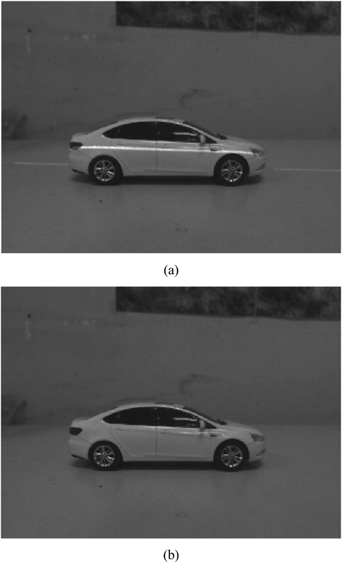
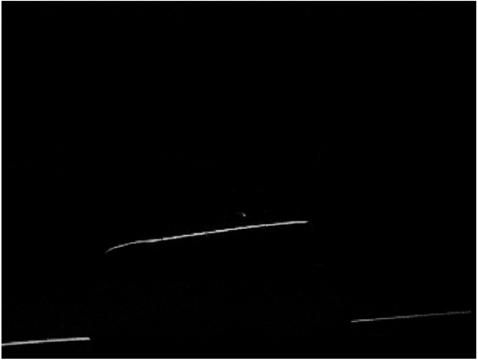
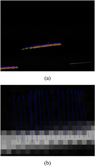
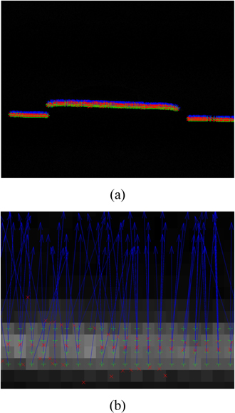
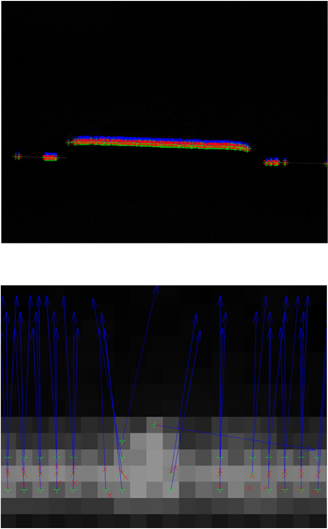
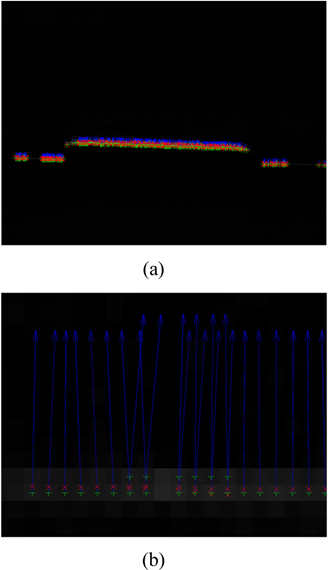
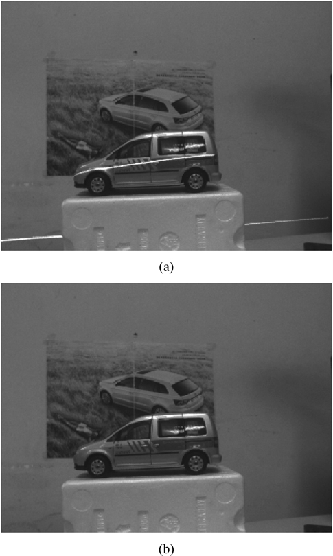
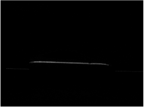
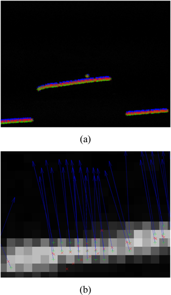
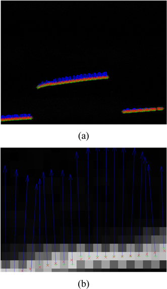
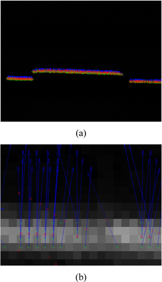
    Figures 1(a) and 2(a) illustrate the target images comprised of the background with an automobile model and a laser line projected onto the surface of the automobile. Figures 1(b) and 2(b) show the backgrounds without the laser lines. The background image is subtracted from the target image to obtain the laser line from the image variation, as shown in Figs. 3 and 4. After image preprocessing, this method removes the irrelevant information such as background, preserves the interesting area with the laser line, and reduces the computation for laser recognition and promotes extraction speed in further steps.

       2.2. Feature Recognition

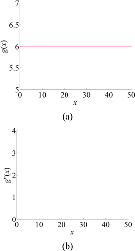
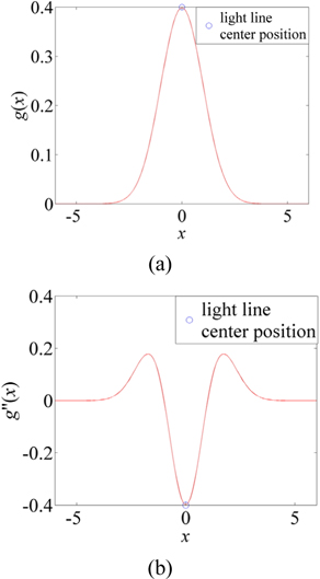
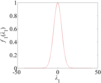
    The Hessian-matrix method was proposed by Steger to extract line centers with good stability [28]. It is composed of second-order partial derivatives of the distribution function of the pixel grayscale values in an image, which expresses the concavity or convexity of the image. Since the crossing line of the laser plane and object surface, which is the laser line, obeys a Gaussian distribution in its transverse section, the second-order partial derivatives of the pixels in different directions should be analyzed to investigate the grayscale distribution characteristics of the laser line in an image [27]. Figure 5(a) explains the variation tendency of gray values along the axis direction of an ideal laser line in an image. Because the variation of gray values is quite small, the partial derivative is approximately regarded as zero, as is interpreted in Fig. 5(b). The variation tendency of gray values along the direction perpendicular to the laser line follows a Gaussian distribution, as shown in Fig. 6(a). The second derivatives of the Gaussian function along the direction perpendicular to the laser line axis are generated to obtain the characteristic of second derivatives of the gray values in this direction, as shown in Fig. 6(b). The second-derivative value related to the center position of the laser line in the transverse section is far less than zero. In conclusion, the rules to determine centers of a laser line are these: The second-order partial derivatives along the central axis of the laser line approach zero, while the second-order partial derivatives along the direction perpendicular to the laser line axis are far less than zero. In other words, the grayscale distribution along the central axis of the laser line is approximately constant, while the grayscale distribution along the direction perpendicular to the laser line axis is a convex function.

    Two eigenvalues of the Hessian matrix respectively express the function's convexity along two orthogonal eigenvectors for any pixel in the image, so the center positions of the laser line can be decided by the characteristics of the two eigenvalues of Hessian matrix. The direction of the laser line is also estimated by the two eigenvectors [31].

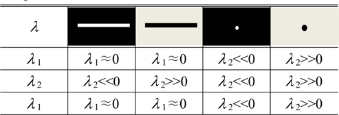
    Table 1 summarizes the relationships between the eigenvalues of the Hessian matrix and the typical grayscale distributions in an image [32]. Whether a pixel is the center of a laser line in an image can be decided if one eigenvalue of the Hessian matrix is close to zero and the other eigenvalue is far less than zero. Obviously, decision rules for other features in Table 1 can be deduced from the above analysis for a laser line.

    [TABLE 1.] Relationships between the eigenvalues λ 1 and λ 2 of the Hessian matrix and typical grayscale distributions in an image

    label

    Relationships between the eigenvalues λ 1 and λ 2 of the Hessian matrix and typical grayscale distributions in an image

    As there is noise in the image, the image Il(x, y) should be convoluted with a Gaussian function to filter the noise. Then the second-order partial derivatives of the convolution result are calculated to obtain the Hessian matrices of the pixels in the image. As the transverse section of a laser line follows a Gaussian distribution, from the differential theorem the convolution result of a laser line image and a Gaussian filter function is still a Gaussian function [33].

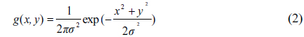
    The Gaussian filter is expressed by

    image

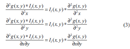
    According to the differential theorem, the convolution results of image Il(x, y) are denoted by

    image

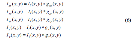
    From Eq. (3), the second-order partial derivatives of the Gaussian function should be calculated first, then the second-order partial derivatives convoluted with the image Il (x, y).

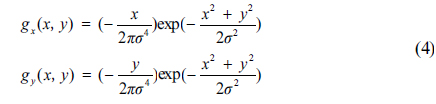
    The first-order partial derivatives of the Gaussian function are expressed by

    image

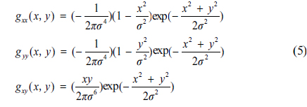
    The second-order partial derivatives of the Gaussian function are denoted by

    image

    Based on Eqs. (4) and (5), the convolution results of the original image and the first-order and second-order derivatives are clarified by Eq. (6) to filter noise in the image.

    image

    where Ixx(x, y), Iyy(x, y), and Ixy(x, y) represent the filtered results of second-order partial derivatives of the Gaussian function with the image Il(x, y) along three directions, and Ix(x, y) and Iy(x, y) are the filtered results of first-order partial derivatives of the Gaussian function with the image Il(x, y) along the x and y directions, respectively.

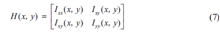
    According to Eq. (6), the Hessian Matrix of an arbitrary pixel in an image is given by

    image

    Suppose λ1 and λ2 are the two eigenvalues of the Hessian matrix and nx and ny are its two eigenvectors. According to the analysis above, if one eigenvalue λ1 approaches zero and the other eigenvalue λ2 is far less than zero, this point is the center point of the laser line. The eigenvector whose direction is related to the eigenvalue close to zero shows the axis direction of the laser line at this point, while the eigenvector whose direction is related to the eigenvalue far less than zero shows the normal to the direction of the laser line at this point [33].

    With this method, two thresholds should be selected to determine the ranges of the two eigenvalues of the Hessian matrix. Too high a threshold leads to losing some center pixels in a laser line, whereas too low a threshold results in more than one center produced in one transverse section of a laser line. To solve this problem, a method for extracting laser line centers is proposed based on a standardized model with a sinusoidal function and a Gaussian fuction. The center positions of a laser line are found by this method.

    III. NORMALIZATION MODEL OF LASER LINE EXTRACTION

    To determine reasonable thresholds for the eigenvalues, a normalization model combining a sinusoidal function and a Gaussian fuction is constructed to extract the laser line centers. First, according to the two eigenvalues of the Hessian matrix, an initial lower threshold is set to choose the preliminary feature points of laser line centers. A lower threshold relatively avoids discontinuous points and completely retains feature pixels of laser line centers. Then, since the gray values are basically constants in the small regions along the axis direction of the laser line, the eigenvalue λ1 of the Hessian matrix associated with the central point in this direction should be close to zero. The Gaussian function f1(λ1) in Eq. (8) is adopted to standardize the judgment numerics for the eigenvalue λ1 in different laser centers. The standardized decision function of the feature points along the central axis of the laser line, as shown in Fig. 7. Its purpose is to assign a large weight to the eigenvalue that is near zero, adjusting the function value to 1 when the eigenvalue λ1 is close to zero.

    image

    where λ1 represents the eigenvalue of the Hessian matrix along the central axis of the laser line, and c is a constant.

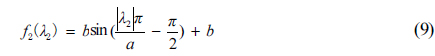
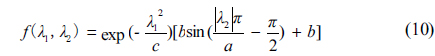
    As the gray values in the direction perpendicular to the central axis of the laser line follows a Gaussian distribution, the eigenvalue λ2 of the Hessian matrix in this direction is far less than zero. The standardized decision function of the feature points perpendicular to the central axis of the laser line, as revealed in Fig. 8. Its aim is to give a large weight to the eigenvalue λ2 that is far less than zero and adapt the function value to 1 when eigenvalue λ2 is far less than zero. To realize standardization for the judgment numerics of different laser centers, the sinusoidal function f2(λ2) in Eq. (9) is adopted.

    image

    where λ2 denotes the eigenvalue of the Hessian matrix perpendicular to the central axis of the laser line, and b is a constant.

    In light of Eqs. (8) and (9), the decision function of the laser line centers based on a sinusoidal function and a Gaussian fuction is given by

    image

    where λ1 and λ2 represent the two eigenvalues of the Hessian matrix. Eigenvalue λ1 is close to zero, and its corresponding eigenvector denotes the central axis direction of the laser line. Eigenvalue λ2 is much smaller than zero, and its related eigenvector shows the direction perpendicular to the central axis of the laser line. For convenience, the absolute value is chosen for λ2 in Eq. (10). f(λ1, λ2) is a standardized model whose value varies from 0 to 1. The eigenvalues of different pixels can be normalized to [0, 1] to regulate differences among the eigenvalues of different pixels. c is a multiple of a. According to the feature of a sinusoidal function passing through the origin and the point [|λ2|, 1], b is determined to 0.5. a is given by Eq. (11)

    image

    where a is the maximum absolute value of eigenvalue λ2 of any of the pixels in the image.

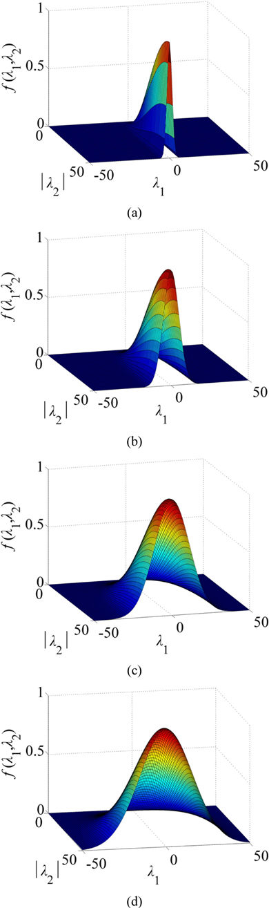
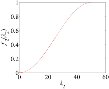
    As elucidated in Fig. 8, the variance ratio of the sinusoidal function increases slowly at both ends but increases quickly in the middle. The benefit is that the resulting distinction is more obvious after the eigenvalues of the different feature points have been substituted into the sinusoidal function. The normalized function provides enormous discrimination between the central and noncentral points. c is an integer multiple of a. Fig. 9 shows the normalization function when c is 0.1a, a, 5a, and 10a in the four diagrams (a), (b), (c), and (d), respectively. The larger the value of c is, the more gently the graph changes. To achieve a high discrimination for a laser line with concentrated brightness, c should take on a small value. For a laser line with scattered brightness, the value of c should be greater. Since the normalization function is composed of two functions, the weight between the two functions in the normalized equation is also an important consideration. c becoming smaller indicates that the weight of the Gaussian function in the normalization equation grows. That means there is more impact on the results from the eigenvalue near zero, which leads to inaccurate extraction of the laser line centers. Moreover, c should not be too large, to avoid redundant points of the laser line centers. The value of c, i.e. the weights of the sinusoidal and Gaussian functions, can be adjusted by experiments. In the following sections the value of c is equal to a.

    In this section, a normalization model integrating a Gaussian recognition function and a sinusoidal recognition function is proposed, to balance the estimation effects on the initiatory laser line centers. The final selected centers are decided by the proposed function, which implies the distribution characteristics of the grayscales along the central axis direction and perpendicular to the central axis direction of the laser line in an image.

    IV. SUBPIXEL EXTRACTION OF LASER LINE CENTERS

    To enhance the accuracy of extraction of the center coordinates of a laser line, the subpixel coordinates of the centers need to be calculated after the pixel coordinates of the laser line have been acquired as in the above sections. As the intensity distribution of the laser line in the transverse section follows a Gaussian distribution, the subpixel coordinates of the laser line centers should be located along the normal direction of the pixel coordinates. In the normal direction, the minimum point of the second-order derivative of the image is the subpixel center of the laser line. Because the direction normal to the laser line is the eigenvector direction corresponding to the minimal eigenvalue of the Hessian matrix, the subpixel coordinates of the laser line centers can be estimated along the normal direction of the central points. In terms of eigenvalues of the Hessian matrix associated with the pixel coordinates of laser line centers, the eigenvector direction related to the minimal eigenvalue, which is the direction normal to the laser line center, can be found. Let (
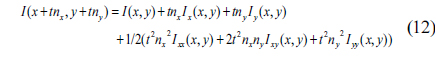
x+tnx, y+tny) be the subpixel coordinate of the center pixel coordinate (x, y) in the normal direction (nx, ny). At the laser line center (x+tnx, y+tny), the second-order Taylor expansion of the grayscale distribution function is given by [27]

    image

    where (x, y) is the center coordinate of a laser line computed with the standardized model; (nx, ny) is the unit vector of a laser line center deduced from the Hessian matrix along the normal direction; Ix(x, y) and Iy(x, y) are the first-order partial derivatives of image I(x, y) along the x and y directions, respectively; Ixx(x, y), Ixy(x, y), and Iyy(x, y) denote the second-order partial derivatives along the x, y, and x-y directions, respectively; and t is the unknown value to be determined.

    As the subpixel point is located on the inflection point in the normal direction, the first-order partial derivative of Eq. (12) is calculated and then set equal to zero [27].
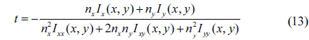
    image

    where Ix(x, y), Iy(x, y), Ixx(x, y), Ixy(x, y), and Iyy(x, y) can be calculated using equation (6), and (nx, ny) is the eigenvector related to the maximal absolute eigenvalues of the Hessian matrix. In this way t can be found with equation (13), then substituted into (x+tnx, y+tny) to obtain the subpixel coordinates of the laser line center.

    V. EXPERIMENTAL RESULTS AND DISCUSSIONS

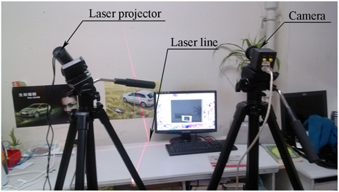
    A vision measurement system of structured light is built to prove the feasibility and accuracy of the outlined standardization model for extracting laser line centers. Experiments on extraction effects of the laser line centers are performed. The experimental system mainly consists of a laser projector, a camera, two tripods, and a computer, as described in Fig. 10. A laser projector with a red laser is used to generate a line on the object's surface. The wavelength of the laser is 635 nm. The camera is DH-HV3102UC-T with the Computar® lens, whose focal length is 5 mm. The image resolution is 640×480. The computer configuration is two 1.6 GHz CPUs and 2 GB of memory.

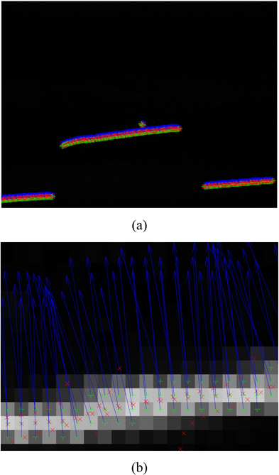
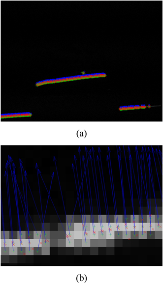
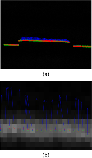
    The difference method is executed to preprocess the first group of images in Fig. 1. The image containing the laser line is shown in Fig. 3. The recognition result and amplified image of the laser line centers extracted by the traditional Hessian matrix method are shown in Fig. 11. The arrows represent the eigenvector directions at the centers perpendicular to the laser line axis. “+” denotes the pixel coordinates of light line centers. “×” denotes the subpixel coordinates of the laser line centers after subpixel analysis. The thresholds are 8 and −8 in Fig. 11. It limits the laser line centers with the conditions that the absolute value of the near−0 eigenvalue λ1 should be smaller than 8, and the eigenvalue λ2 which is far less than 0 should be smaller than −8. It reveals that several redundant centers appear on the same transverse section of the laser line. To avoid extracting several center points, the experiment in Fig. 12 decreases the threshold for λ1 from 8 to 3; the threshold for λ2 is still −8. It can be observed from Fig. 12 that laser line centers are missed in some transverse sections, while multiple laser line centers are extracted in some of the transverse sections. The thresholds for λ1 and λ2 are respectively set to 8 and −15 to filter the centers with absolute value of eigenvalue λ1 larger than 8 or absolute value of eigenvalue λ2 smaller than 15. As described in Fig. 13, the results still include excess center points, and several points are missed in the transverse sections. The thresholds for λ1, λ2 are next narrowed to 3, −37. The results are shown in Fig. 14. It can be seen from the image that the center extraction effects in the left and middle of the image are better than for the previous group. However, the laser line centers on the right of Fig. 14(a) are lost. Consequently, the traditional Hessian matrix method cannot accurately extract laser line centers as the result of the limit of threshold selection. The centers image and amplified image of the laser line obtained from the center extraction method based on the standardized model are shown in Fig. 15. Each column of the laser line is scanned and the standardized function values of the laser line centers are calculated in this experiment. The pixel with the maximum value of the standardized function is chosen as the laser line center in the column. Figures 16, 17, 18, and 19 are the center images and amplified images of the laser line centers extracted by the Hessian matrix method with different thresholds for the second group of images in Fig. 2. It can be seen that there are also the same problems as for the results of the first test group. Figures 20 are the centers image and amplified image of the laser line generated from the center extraction method based on the standardized model for the second group in Fig. 2. Figures 14 and 19 are chosen as the samples of the traditional method, considering that their results are better than the other three images in their group. The left bottom part of the laser line in the image is selected as the statistical object. 100 continuous pixel centers of the laser line are calculated in the experiment. In the first group, 60 centers in the laser line are recognized correctly. However, 40 centers failed to be identified, including 31 redundant centers, 4 missed centers, and 5 deviated centers. The number of recognition centers of the proposed method is 86 in Fig. 15, so the recognition rate of the proposed method is 26% higher than for the traditional method. In the second group, 51 correct centers are found by the traditional method while 43 redundant centers and 6 missed centers are also observed in the experimental image. Using the proposed method, the number of recognized centers is 89, also higher than with the traditional method. Compared to the extraction results of the laser line centers using the traditional method, the normalized model provides a decision function to balance the two eigenvalues of the candidate centers in the laser line. The decision function enhances the judgment performance for laser line centers based on the characteristic of grayscale distribution in the longitudinal and transverse directions of the laser line. Owing to the unitary value of the decision function for one candidate center, the situations of losing center points or extracting several center points in the same transverse section are avoided in the column scan. Based on the more reliable pixel-level coordinates, the subpixel coordinates of laser line centers can be extracted precisely.

    VI. CONCLUSIONS

    To improve the extraction stability of laser line centers in active vision, an extraction method for laser line centers based on a standardized model with a sinusoidal function and a Gaussian function is presented. First, preprocessing of the camera-captured image with a difference method is conducted to segment the laser line from the complex background image. Then the eigenvalues and eigenvectors of the Hessian matrix are calculated after obtaining the Hessian matrix of each pixel on the laser line. Thresholds are acquired according to the characteristics of the Hessian matrix eigenvalues of laser line centers that follow a Gaussian distribution, which is used to select the initial laser line centers. Third, combining the characteristics of a sinusoidal recognition function and a Gaussian recognition function, a standardized model of eigenvalues for the Hessian matrix is constructed to extract laser line centers accurately. In the proposed model the sinusoidal recognition function corresponds to the Gaussian distribution of the laser line in transverse section and assigns a larger weight to the real center that has a negative eigenvalue with a large absolute value. The Gaussian recognition function explains the constant distribution of the laser line in longitudinal section and gives a larger weight to the center with eigenvalue close to zero. The advantage of this model for constructing a normalized decision function is to identify the real centers from the candidate centers. In the decision function of the model, if one eigenvalue of the Hessian matrix at the pixel point is close to 0 and the other one is much less than 0, the normalized result is near 1. In other conditions, the standardized result approaches 0. Therefore, the former decision basis which depends on the eigenvalues is legitimately standardized to the interval between 0 and 1 by the decision function, which supplies a unitary decision value to improve the recognition rate of the laser line centers in different images. Finally, a comparative experiment is completed with the traditional method. The experiments put the two eigenvalues of the Hessian matrix into the standardized model. The maximum points of standardization results in each column are adopted as laser line centers. The foundation that balances the two eigenvalues of Hessian matrix is presented for the process of determining the laser line centers. The subpixel level results of center coordinates of the laser line are found. For 100 continuous centers of a laser line in two group images, the proposed method increases the recognition rate of two image groups from 60% to 86% and from 51% to 89% compared to the former method. The experimental results show that the normalization method that integrates the Gaussian and sinusoidal recognition functions elucidates the distribution characteristic of laser line centers and improves the extraction accuracy for the coordinates of laser line centers.

참고문헌
  • 1. Joo W. D. 2011 Analysis of specific problems in laser scanning optical system design [J. Opt. Soc. Korea] Vol.15 P.22-29 google
  • 2. Brown E. B., Campbell R. B., Tsuzuki Y., Xu L., Carmeliet P., Fukumura D., Jain R. K. 2001 In vivo measurement of gene expression angiogenesis and physiological function in tumors using multiphoton laser scanning microscopy [J. Nat. Med.] Vol.7 P.864-868 google
  • 3. Cho M., Shin D. 2013 Depth resolution analysis of axially distributed stereo camera systems under fixed constrained resources [J. Opt. Soc. Korea] Vol.17 P.500-505 google
  • 4. Walecki W. J., Szondy F., Hilali M. M. 2008 Fast in-line surface topography metrology enabling stress calculation for solar cell manufacturing for throughput in excess of 2000 wafers per hour [Meas. Sci. Technol.] Vol.19 P.025302 google
  • 5. Son T., Lee J., Jung B. 2013 Contrast enhancement of laser speckle contrast image in deep vasculature by reduction of tissue scattering [J. Opt. Soc. Korea] Vol.17 P.86-90 google
  • 6. Jo T. Y., Kim S. Y., Pahk H. J. 2013 3D measurement of TSVs using low numerical aperture white-light scanning interferometry [J. Opt. Soc. Korea] Vol.17 P.317-322 google
  • 7. Liu K., Wang Y. C., Lau D. L., Hao Q., Hassebrook L. G. 2010 Dual-frequency pattern scheme for high-speed 3-D shape measurement [Opt. Express] Vol.18 P.5229-5244 google
  • 8. Song B., Min S. W. 2013 2D/3D convertible integral imaging display using point light source array instrumented by polarization selective scattering film [J. Opt. Soc. Korea] Vol.17 P.162-167 google
  • 9. Goel S., Lohani B. 2014 A Motion correction technique for laser scanning of moving objects [IEEE Geosci. Remote S.] Vol.11 P.225-228 google
  • 10. Larsson S., Kjellander J. A. P. 2006 Motion control and data capturing for laser scanning with an industrial robot [Robot. Auton. Syst.] Vol.54 P.453-460 google
  • 11. Duffy N. D., Yau J. F. S. 1988 Facial image reconstruction and manipulation from measurements obtained using a structured lighting technique [Pattern Recogn. Lett.] Vol.7 P.239-243 google
  • 12. Moss J. P., Linney A. D., Grindrod S. R., Mosse C. A. 1989 A laser scanning system for the measurement of facial surface morphology [Opt. Laser. Eng.] Vol.10 P.179-190 google
  • 13. Tsujimura T., Minato Y., Izumi K. 2013 Shape recognition of laser beam trace for human-robot interface [Pattern Recogn. Lett.] Vol.34 P.1928-1935 google
  • 14. Pinto A. M., Rocha L. F., Moreira A. P. 2013 Object recognition using laser range finder and machine learning techniques [Robot. Cim.-Int. Manuf.] Vol.29 P.12-22 google
  • 15. Canny J. 1986 A computational approach to edge detection [IEEE. T. Pattern Anal.] Vol.6 P.679-698 google
  • 16. Perona P., Malik J. 1990 Scale-space and edge detection using anisotropic diffusion [IEEE. T. Pattern Anal.] Vol.12 P.629-639 google
  • 17. Harris C., Stephens M. 1988 A combined corner and edge detector [Proc. Alvey Vision Conference] P.147-151 google
  • 18. Weijer J. V. D., Gevers T., Geusebroek J. M. 2005 Edge and corner detection by photometric quasi-invariants [IEEE. T. Pattern Anal.] Vol.27 P.625-630 google
  • 19. Tsai L. W., Hsieh J. W., Fan K. C. 2007 Vehicle detection using normalized color and edge map [IEEE T. Image Process.] Vol.16 P.850-864 google
  • 20. Chaudhuri S., Chatterjee S., Katz N., Nelson M., Goldbaum M. 1989 Detection of blood vessels in retinal images using two-dimensional matched filters [IEEE T. Med. Imaging] Vol.8 P.263-269 google
  • 21. Ziou D. 1991 Line detection using an optimal IIR filter [Pattern Recogn.] Vol.24 P.465-478 google
  • 22. Laligant O., Truchetet F. 2010 A nonlinear derivative scheme applied to edge detection [IEEE. T. Pattern Anal.] Vol.32 P.242-257 google
  • 23. Shortis M. R., Clarke T. A., Short T. 1994 A comparison of some techniques for the subpixel location of discrete target images [Proc. SPIE] Vol.2350 P.239-250 google
  • 24. Luengo-Oroz M. A., Faure E., Angulo J. 2010 Robust iris segmentation on uncalibrated noisy images using mathematical morphology [Image Vision Comput.] Vol.28 P.278-284 google
  • 25. Xu G. S. 2009 Sub-pixel edge detection based on curve fitting [Proc. The Second International Conference on Information and Computing Science] P.373-375 google
  • 26. Goshtasby A., Shyu H. L. 1995 Edge detection by curve fitting [Image Vision Comput.] Vol.13 P.169-177 google
  • 27. Steger C. 1998 An unbiased detector of curvilinear structures [IEEE. T. Pattern Anal.] Vol.20 P.113-125 google
  • 28. Qi L., Zhang Y., Zhang X., Wang S., Xie F. 2013 Statistical behavior analysis and precision optimization for the laser stripe center detector based on Steger’s algorithm [Opt. Express] Vol.21 P.13442-13449 google
  • 29. Lemaitre C., Perdoch M., Rahmoune A., Matas J., Miteran J. 2011 Detection and matching of curvilinear structures [Pattern Recogn.] Vol.44 P.1514-1527 google
  • 30. Alard C., Lupton R. H. 1998 A method for optimal image subtraction [Astrophys. J.] Vol.503 P.325-331 google
  • 31. Steger C. 2012 Unbiased extraction of lines with parabolic and Gaussian profiles [Comput. Vis. Image Und.] Vol.117 P.97-112 google
  • 32. Frangi A. F., Niessen W. J., Hoogeveen R. M., Walsum T. V., Viergever M. A. 1999 Model-based quantitation of 3-D magnetic resonance angiographic images [IEEE T. Med. Imaging] Vol.18 P.946-956 google
  • 33. Steger C. 1996 Extracting curvilinear structures: A differential geometric approach [Proc. Computer Vision-ECCV'96] P.630-641 google
OAK XML 통계
이미지 / 테이블
  • [ ] 
  • [ FIG. 1. ]  The first example of a measured object: (a) Target image, (b) Background image.
    The first example of a measured object: (a) Target image, (b) Background image.
  • [ FIG. 2. ]  The second example of a measured object: (a) Target image, (b) Background image.
    The second example of a measured object: (a) Target image, (b) Background image.
  • [ FIG. 3. ]  Laser line image of the first example.
    Laser line image of the first example.
  • [ FIG. 4. ]  Laser line image of the second example.
    Laser line image of the second example.
  • [ FIG. 5. ]  (a) The variation tendency of gray values along the axis direction of an ideal laser line. (b) The second-order derivative of (a).
    (a) The variation tendency of gray values along the axis direction of an ideal laser line. (b) The second-order derivative of (a).
  • [ FIG. 6. ]  (a) The variation tendency of gray values along the vertical direction of the laser line. (b) The second-order derivative of (a).
    (a) The variation tendency of gray values along the vertical direction of the laser line. (b) The second-order derivative of (a).
  • [ TABLE 1. ]  Relationships between the eigenvalues λ 1 and λ 2 of the Hessian matrix and typical grayscale distributions in an image
    Relationships between the eigenvalues λ 1 and λ 2 of the Hessian matrix and typical grayscale distributions in an image
  • [ ] 
  • [ ] 
  • [ ] 
  • [ ] 
  • [ ] 
  • [ ] 
  • [ Fig. 7. ]  The standardized decision function of the feature points along the central axis of the laser line, f1 (λ1).
    The standardized decision function of the feature points along the central axis of the laser line, f1 (λ1).
  • [ ] 
  • [ Fig. 8. ]  The standardized decision function of the feature points perpendicular to the central axis of the laser line, f2 (λ2).
    The standardized decision function of the feature points perpendicular to the central axis of the laser line, f2 (λ2).
  • [ ] 
  • [ ] 
  • [ ] 
  • [ FIG. 9. ]  The normalization function of the eigenvalues λ1 and λ2 of the Hessian matrix for the laser line, f (λ1, λ2): (a) c = 0.1a, (b) c = a, (c) c = 5a, (d) c = 10a.
    The normalization function of the eigenvalues λ1 and λ2 of the Hessian matrix for the laser line, f (λ1, λ2): (a) c = 0.1a, (b) c = a, (c) c = 5a, (d) c = 10a.
  • [ ] 
  • [ ] 
  • [ FIG. 10. ]  The experimental measurement system with a laser line.
    The experimental measurement system with a laser line.
  • [ FIG. 11. ]  The recognition result and amplified image of the laser line centers in Fig. 3 extracted by the traditional Hessian-matrix method. The threshold for λ1 is 8 and the threshold for λ2 is ?8. (a) Original image, (b) Amplified image.
    The recognition result and amplified image of the laser line centers in Fig. 3 extracted by the traditional Hessian-matrix method. The threshold for λ1 is 8 and the threshold for λ2 is ?8. (a) Original image, (b) Amplified image.
  • [ FIG. 12. ]  The recognition result and amplified image of the laser line centers in Fig. 3 extracted by the traditional Hessian-matrix method. The threshold for λ1 is 3 and the threshold for λ2 is ?8. (a) Original image, (b) Amplified image.
    The recognition result and amplified image of the laser line centers in Fig. 3 extracted by the traditional Hessian-matrix method. The threshold for λ1 is 3 and the threshold for λ2 is ?8. (a) Original image, (b) Amplified image.
  • [ FIG. 13. ]  The recognition result and amplified image of the laser line centers in Fig. 3 extracted by the traditional Hessian-matrix method. The threshold for λ1 is 8 and the threshold for λ2 is ?15. (a) Original image, (b) Amplified image.
    The recognition result and amplified image of the laser line centers in Fig. 3 extracted by the traditional Hessian-matrix method. The threshold for λ1 is 8 and the threshold for λ2 is ?15. (a) Original image, (b) Amplified image.
  • [ FIG. 14. ]  The recognition result and amplified image of the laser line centers in Fig. 3 extracted by the traditional Hessian-matrix method. The threshold for λ1 is 3 and the threshold for λ2 is ?37. (a) Original image, (b) Amplified image.
    The recognition result and amplified image of the laser line centers in Fig. 3 extracted by the traditional Hessian-matrix method. The threshold for λ1 is 3 and the threshold for λ2 is ?37. (a) Original image, (b) Amplified image.
  • [ FIG. 15. ]  The centers image and amplified image of the laser line in Fig. 3 obtained from the center extraction method based on the normalization model. (a) Original image, (b) Amplified image.
    The centers image and amplified image of the laser line in Fig. 3 obtained from the center extraction method based on the normalization model. (a) Original image, (b) Amplified image.
  • [ FIG. 16. ]  The recognition result and amplified image of the laser line centers in Fig. 4 extracted by the traditional Hessian-matrix method. The threshold for λ1 is 3 and the threshold for λ2 is ?3. (a) Original image, (b) Amplified image.
    The recognition result and amplified image of the laser line centers in Fig. 4 extracted by the traditional Hessian-matrix method. The threshold for λ1 is 3 and the threshold for λ2 is ?3. (a) Original image, (b) Amplified image.
  • [ FIG. 17. ]  The recognition result and amplified image of the laser line centers in Fig. 4 extracted by the traditional Hessian-matrix method. The threshold for λ1 is 1 and the threshold for λ2 is ?3. (a) Original image, (b) Amplified image.
    The recognition result and amplified image of the laser line centers in Fig. 4 extracted by the traditional Hessian-matrix method. The threshold for λ1 is 1 and the threshold for λ2 is ?3. (a) Original image, (b) Amplified image.
  • [ FIG. 18. ]  The recognition result and amplified image of the laser line centers in Fig. 4 extracted by the traditional Hessian-matrix method. The threshold for λ1 is 3 and the threshold for λ2 is ?6. (a) Original image, (b) Amplified image.
    The recognition result and amplified image of the laser line centers in Fig. 4 extracted by the traditional Hessian-matrix method. The threshold for λ1 is 3 and the threshold for λ2 is ?6. (a) Original image, (b) Amplified image.
  • [ FIG. 19. ]  The recognition result and amplified image of the laser line centers in Fig. 4 extracted by the traditional Hessian-matrix method. The threshold for λ1 is 1 and the threshold for λ2 is ?5. (a) Original image, (b) Amplified image.
    The recognition result and amplified image of the laser line centers in Fig. 4 extracted by the traditional Hessian-matrix method. The threshold for λ1 is 1 and the threshold for λ2 is ?5. (a) Original image, (b) Amplified image.
  • [ FIG. 20. ]  The centers image and amplified image of the laser line in Fig. 4 obtained from the center extraction method based on the normalization model. (a) Original image, (b) Amplified image.
    The centers image and amplified image of the laser line in Fig. 4 obtained from the center extraction method based on the normalization model. (a) Original image, (b) Amplified image.
(우)06579 서울시 서초구 반포대로 201(반포동)
Tel. 02-537-6389 | Fax. 02-590-0571 | 문의 : oak2014@korea.kr
Copyright(c) National Library of Korea. All rights reserved.