Although bottom fixed breakwaters have an advantage in calming harbors, there are some problems with water pollution in the harbors due to the blockage of currents, moreover, the cost of construction increases considerably in deep sea or soft ground conditions. Floating breakwaters can be an alternative, but they have poorer performance than bottom fixed breakwaters. In addition, disaster can occur if the mooring lines are damaged (Lee and Song, 2005). To increase the performance of a breakwater, the effects of nonlinear phenomena, such as overtopping and breaking waves need to be analyzed. To secure the safety of mooring lines, the maximum tensions on the mooring lines have to be estimated considering the second order wave drift force on a floating breakwater.

The motion of a floating body has been analyzed mostly based on potential theory. Most studies of floating breakwaters were also performed based on potential theory (Loukogeorgaki and Angelides, 2005; Lee and Cho, 2003; Lee and Song, 2005; Song and Kim, 2005). The potential theories use linearized governing equations and free surface boundary conditions. The theories, however, show satisfactory results when linear assumptions are suitable for the purpose only. If the flows include highly nonlinear phenomena such as wave breaking and wave overtopping, the potential theories cannot produce meaningful results. Because such nonlinear phenomena are not negligible estimating the performance and evaluating the safety of mooring lines, a method that can analyze nonlinear phenomena is necessary. Experiments are an alternative method, and there have been performed many researchers (Ruol et al., 2008; Chun and Cho, 2011). Computational Fluid Dynamics (CFD) can be another alternative method. Koftis and Prinos (2005) examined flow near a floating breakwater using the CFD. In Koftis and Prinos (2005), the motions of the breakwater were not considered. The motions should be considered in the analysis to obtain more rational results. A grid technique for a moving body and a free surface model for a nonlinear wave are important. The grid system is essential in most numerical simulations for practical purposes even though there are meshless methods using particle such as Najafi-Jilani and Rezaie-Mazyak (2011) and Jung et al. (2008). The grid systems have been categorized in two groups; a body fitted grid system and a non-body fitted Cartesian grid system (Mittal and Iaccarino, 2005). The body fitted grid system provides a more accurate result particularly near the body boundary. Many research using body fitted grid have been conducted for floating body in waves with grid deformation, overset grid or grid regeneration (Guo et al., 2012; Sadat-Hosseini et al., 2013; Hadzic et al., 2005; Simonsen et al., 2013). In body fitted grid system, grid generation near a complex body requires considerable time and effort. Moreover, grid regeneration and interpolation between overset grids for moving a body take huge time. On the other hand, the Cartesian grid system has advantages on easy grid generation and fast calculation. In the Cartesian grid system, the grid lines do not consist with the body surface. Therefore, a special treatment is required for a body boundary treatment. These methods are called the Immersed Boundary Method (IBM). The greatest advantage of the Cartesian grid is the easy treatment of moving bodies in a fixed grid system. A range of methods for a moving body in a Cartesian grid system have been developed. On the other hand, few methods consider the problems including the free surface. Normally, zero gradient boundary conditions are imposed for pressure and velocity on the body boundary. These boundary conditions are difficult to be satisfied if a body boundary cell contains the free surface, due to the drastic differences in the densities and viscous coefficients. Lin (2007) proposes the Partial Cell Treatment (PCT) method to simulate a moving body on the free surface. The PCT method defines the body boundary using the volume ratio in a cell between the body and fluid. Therefore, the PCT method cannot define the body surface as sharply as the Ghost Cell Immersed Boundary Method (GCIBM) and Cartesian Cut Cell (CCM) (Hu and Kashiwagi, 2009). In the present study, a body boundary treatment technique using no-slip and divergence free conditions is suggested for the sharp definition of the body boundaries.

The differences in the densities and viscous coefficients of water and air are sources of solution instability. The most popular method for free surface modeling is the Volume of Fluids (VOF) method (Hirt and Nichols, 1981). In the VOF method, the free surface is treated as a transient zone, where the density and viscosity varies continuously in space. The densities and viscous coefficients of the cells near the free surface are defined using the volume fractional function. The transient zone is a source of the reduction of the accuracy of the solution. Park et al. (1999) proposed the marker-density method, which does not use transient zone. To obtain the sufficient stability, the velocities of air in the free surface cells are extrapolated from the water velocities. Lee et al. (2012) suggested the modified marker-density method which calculates the velocities of air in the free surface cells with the governing equations. In this study, the modified marker-density method is implemented for the nonlinear free surface definition.

To verify developed numerical method, vortex induced vibrations on the elastically mounted circular cylinder are numerically simulated and the results are compared with the results of other researches. Moreover, a free roll decay simulation is performed and the results are compared with the data in the published literature. Finally, three kinds of breakwaters in regular wave are simulated using the present numerical method.

The filtered Navier-Stokes equations and the continuity equation are employed as governing equations. Subgrid-scale (SGS) turbulence model is implemented to consider the effects of the turbulence flow smaller than a grid. f_i in Eq. (1) denotes the gravitational acceleration and r_ij is SGS Reynolds stress.

The governing equations are descretized with Foreword Time, Centred Space (FTCS) except for convection terms. The convection terms are descretized using the Kawamura-Kuwahara scheme (Kawamura and Kuwahara, 1984) and first order upwind scheme considering the number of fluid cells in space and the Adams-Bashforth scheme in time. The descretized governing equation is shown in Eqs. (3) and (4).

where represents a discretized spatial derivation and u^* denotes the tentative velocity in Eq. (5).

By substituting Eq. (3) into Eq. (4), the pressure Poisson equation Eq. (6) is obtained and the pressure Poisson equation is solved using the Successive Over Relaxation method. More details of spatial descretization can be found in Lee et al. (2012).

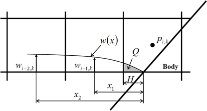
The governing equations are solved in a staggered Cartesian grid. Because the grid line does not consist with the body surface, the body boundaries are defined by line segments connecting the points where the grid line and body surface meet. The grids containing the line segment are defined as body boundary cell. The no-slip condition is imposed on the body surface and the zero-divergence condition is imposed in body boundary cell. The velocity near a body is assumed to follow a quadratic polynomial w(x) in Fig. 1. Inducing the velocity profile, '0' is imposed on the body surface for the no-slip boundary condition.

To satisfy the divergence free condition, the divergence of a body boundary cell is calculated by joining the fluxes passing through the grid lines together. The flux Q (in Fig. 1) through the grid line of the cut cell H is calculated by integrating the quadratic polynomial. Using the divergence, new pressures are calculated in Eq. (7), and the velocities are computed from them using Eq. (3). The superscripts in Eq. (7) mean the inner iteration steps. Until the pressures and velocities are converged, the iterative calculation continues to satisfy the zero-divergence condition.

where D is the divergence of body boundary cells, and ω is the relaxation factor.

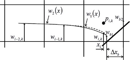
When a body moves, velocity profiles are induced with the velocities of the body surface ( w_b1 in Fig. 2) instead of the zero value in Fig. 1. The velocity profiles for the flux calculation change abruptly when the body surface passes the velocity definition point in a certain time interval because the velocity definition points used for the velocity profiles change. This causes spurious pressure oscillations. To prevent the abrupt change in the volume flux through the grid face, the volume flux is determined with the weighted average of the two fluxes according to Eq. (8). Q₁ and Q₂ are obtained by integrating the velocity profile w₁ (x) and w ₂(x) , respectively. The velocity profile w₁ (x) is induced with w_b1 , w_{i −1},_k, and w_{i −2},_k , and the velocity profile w₂ (x) is induced with w_b1 , w_{i, k}, and w_{i −1}, _k.

Eq. (9) must be satisfied to conserve the mass in a body boundary cell. A_B is the area occupied by the body in a cell. The second term in Eq. (9) is calculated by adding all fluxes together through grid faces. Instead of calculating A _B, the amount of the body passing through the face is added to the volume flux as shown in Eq. (10) for an easy calculation of the first term of Eq. (9). Eq. (10) cannot substitute for Eq. (9) sufficiently if the body shape change sharply like a corner.

If a fluid cell neighboring the body boundary undergoes a change to become a body boundary cell, the pressure changes abruptly because the pressure calculation undergoes a different process according to the change in the geometrical surrounding. In this case, the pressure in the fluid cell neighboring the body boundary cell can be determined using the same process that is applied to the body boundary cell described in previous paragraphs.

Eqs. (11) and (12) show the dynamic and kinematic boundary conditions of the free surface. Eq. (11) means that the air pressure is the same as that of water on the free surface and the surface tension and the viscous stress on free surface are ignored. Eq. (12) means that the velocities of a fluid particle and the free surface normal to the free surface are the same on that location of the free surface.

In the above, and mean the velocity vectors of the fluid particle and free surface respectively, and stands for the normal vector of the free surface.

The transport equation of the Marker-density is used to define the position of the free surface, as shown in Eq. (13) instead of Eq. (12). The value of the Marker-density is an artificial density obtained numerically from the water density ( ρ_water ) and air density ( ρ_air ). A cell is considered to be a water cell if the Marker-densities of a cell and its neighboring cells are larger than the average of the air and water densities. On the other hand, the cell is considered an air cell if the Marker-densities of a cell and its neighboring cells are less than the average of the air and water densities. Other fluid cells are treated as free surface cells. The location of the free surface is determined where the Marker-density is the average of the air and water densities.

The method for the free-surface definition is similar to the VOF method. In the VOF method, the volume fraction is used to determine the density and viscosity of the free surface cell. The velocity and pressure of free surface cells are calculated using the weighted average density and viscosity by a volume fraction. In the Marker-density method, on the other hand, the air and water regions are treated as separate regions. Therefore, the Marker-density value is used only to define the free surface position. In this study, the pressure and velocity distributions are calculated from the density and the viscosity of air or water, not from the Marker-density.

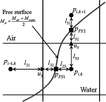
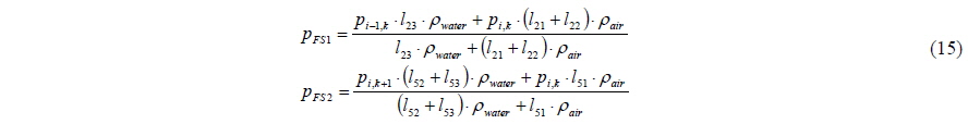
In the traditional Marker-density method, the pressure on the free surface is extrapolated equally from the nearest air cell including gravitational acceleration. Also the air velocity of free surface cell is extrapolated with Lagrangian manner to obtain the stability of the solutions (Park et al., 1999). In the present method, on the other hand, the air velocity of free surface cell is calculated with governing equations. For the stability of the solution, continuous pressure gradient condition (Eq. (14)) is additionally imposed. Fig. 3 and Eq. (15) show how to calculate the pressure on the free surface.

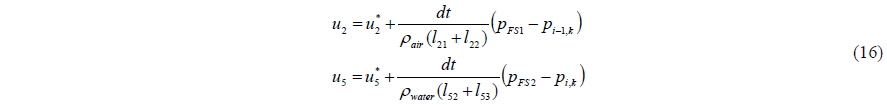
The velocities and pressures of the free surface cells are calculated using a simultaneous iteration method. The velocities of the free surface cells are calculated according to Eq. (16). and in Eq. (16) are the tentative velocities in Eq. (5). The divergences of free surface cells are calculated using the velocities of the free surface. The pressure is updated or calculated at each inner iteration step with the new divergence according to Eq. (7). Until the pressures and velocities converge, they are calculated iteratively.

The process to obtain the pressure and velocity of body boundary and free surface cells are identical. Therefore, additional treatment is not necessary to get the stability of the body boundary cell including the free surface.

Velocity distribution of the Stokes's 2nd order wave theory is imposed on the inflow boundary to generate regular waves. Neumann boundary condition is imposed for the pressure and wave elevation on the inflow boundary. To prevent unintended wave reflection or pressure oscillation on the outflow boundary, artificial damping zone is imposed near the outflow boundary. As shown in Eq. (17), the velocity of z- direction are artificially damped 1% every time step.

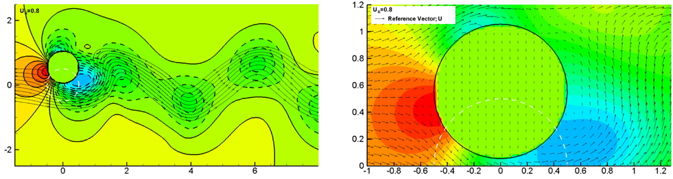
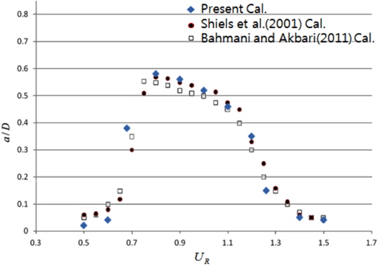
Vortex shedding on the circular cylinder suspended by an elastic spring is simulated numerically at Re = 100. The SGS turbulence model is not employed in these calculations due to the low Reynolds number. The amplitude and period of the cylinder motion are affected by the mass of cylinder (m) and spring constant (k). The mass ratio (m^* = 4m/πρD²L ) is 5 and the non-dimensional velocities ( ) ranged from 0.5 to 1.5.

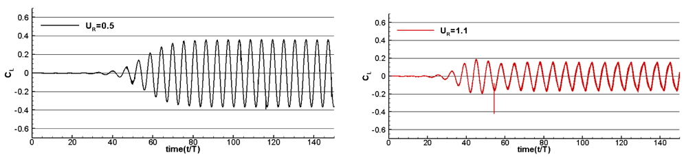
Fig. 4 shows the amplitude of oscillating cylinder at various non-dimensional velocities. The present calculation results agree with the other research data of Bahmani and Akbari (2011) and Shiels et al. (2001). A 'Lock-in' phenomenon, in which the period of vortex shedding coincides with the period of the mass spring system are observed from 0.8 to 1.1 of the nondimensional velocity. Fig. 5 shows the time histories of lift force coefficient of the cylinder in U_R= 0.5 and U_R=1.1 conditions. Even though, there are several spurious pressure oscillations, the effects are small enough to ignore. Fig. 6 shows the pressure contours, stream lines and velocity vectors near the moving cylinder. In the figure the dashed lines indicate the initial position of the cylinder. The velocity vectors in the cylinder mean the velocity of the moving cylinder. Fig. 6 shows the spatially continuous variation of velocity and pressure. The present numerical simulation method is applicable to the simulation of translational body motion by fluid force.

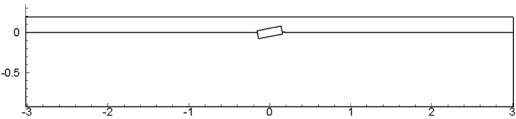
Using a rectangular floating body, a free roll decay test is performed to check the applicability to the problem including the free surface. The breadth of the body is 0.3m and the draft is 0.05m. The translational movements are restrained and the rotational movement is set free. The moment of inertia is equal to 0.262kg/m². The SGS turbulence model is implemented in the calculation. The initial roll angle is set 15°. Fig. 7 shows the calculation domain. Three grid size cases (0.004m, 0.002m, and 0.001m) are employed to check the grid dependency and the time interval is set to 5/10000_s.

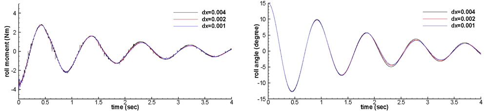
Fig. 8 presents the time histories of the roll moment and roll angle. In the case of a grid size of 0.004m, there are spiky variations in the moment history. On the other hand, the roll moment variations are smooth in the case of a grid size of 0.002m and 0.001m. In the case of a grid size of 0.004m, the roll angle is different from other cases. Between the cases of grid sizes of 0.002m and grid size 0.001m, there are small differences that could be ignored.

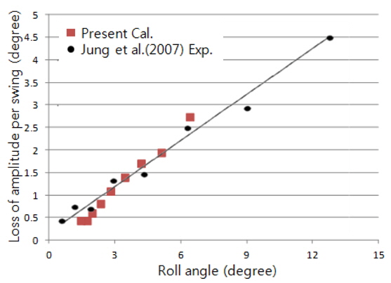
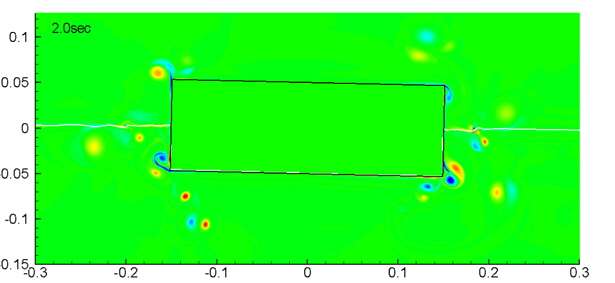
The results of the present simulation are compared with the experimental data reported in Jung et al. (2007) in Fig. 9. The agreement is sufficient to apply the present method to simulate the rotational motion of a floating body when the roll angle is smaller than 6°. Fig. 10 shows the vorticity distribution near the floating body. A number of vortexes exist near the body and affect the motion of the body.

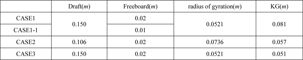
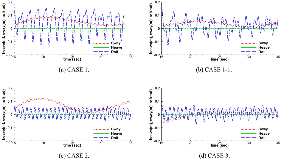
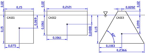
Three breakwater shapes are investigated under the same displacement. The shape of the submerged area of CASE 1 is a square shape with 0.15m edges. The ratio between the breadth and draft of CASE 2 is equal to 2. CASE 3 is designed by giving a slope to the side walls of CASE 1. Fig. 11 shows the shape of each case. Table 1 lists the principal dimensions of all the cases.

To investigate the effects of wave overtopping, CASE 1-1, which is designed by reducing the freeboard of CASE 1, is additionally simulated. To limit the drift due to waves, it is assumed that all the breakwaters are moored by linear spring in the x- direction. The spring constant is set to 2N/m. The length of incident wave is 0.75m and the height is 0.030m.

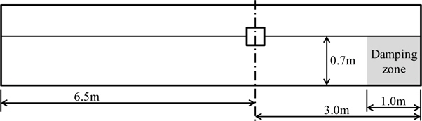
Fig. 12 shows the schematic sketch for the calculation domain. The calculations cannot continue after the waves reflected by the breakwater reaches the inflow boundary. Therefore, the inflow boundary is located sufficiently far from the floating breakwater. A damping zone is placed near the end of the computational domain to avoid unintended reflections by the outflow boundary. The minimum grid sizes in the x- and z- directions are 0.002m. The time interval is equal to 4/10,000_s.

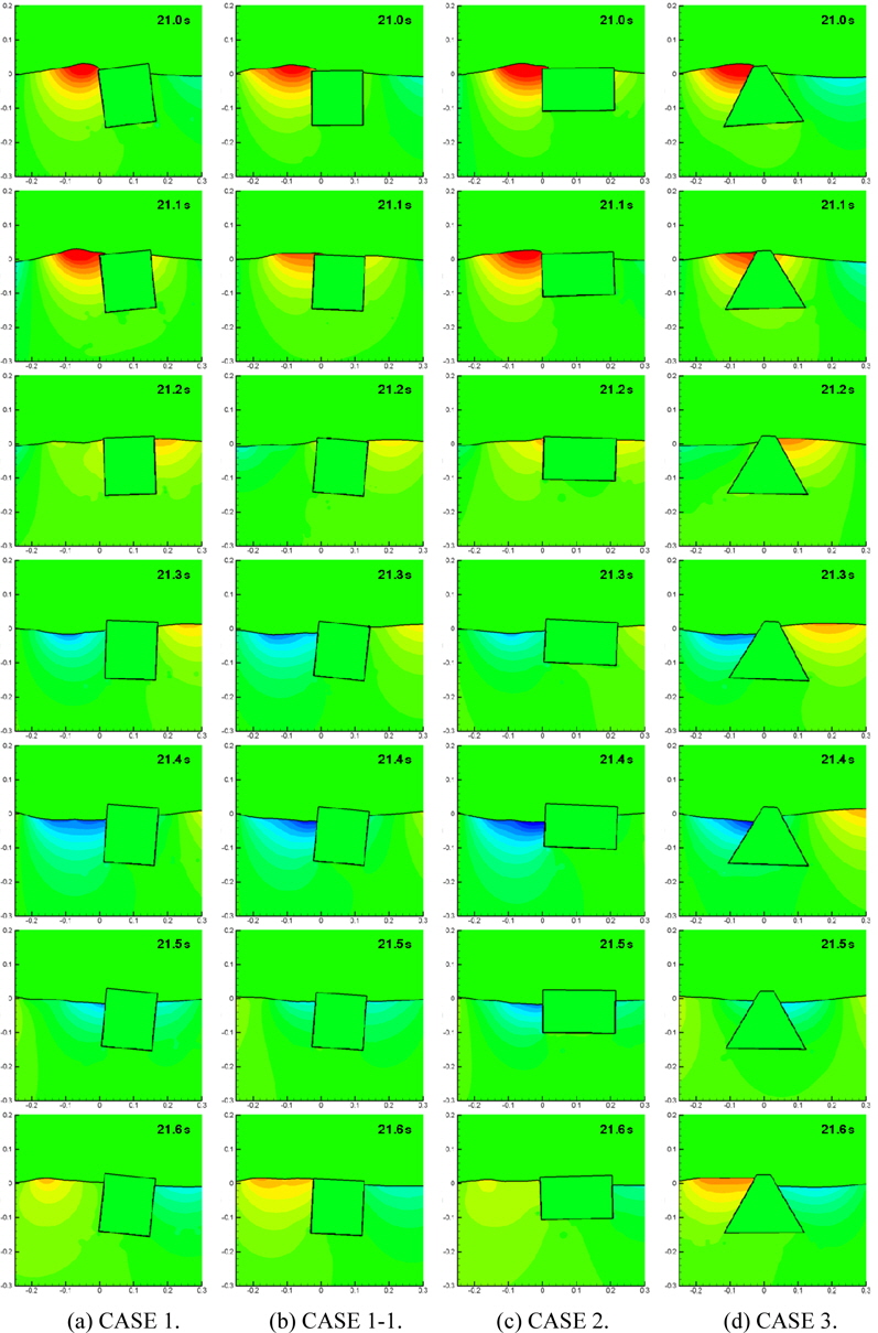
Fig. 13 shows the pressure distributions around each breakwater from 21.0_s to 22.6_s. The pressure distributions around CASE 1 are similar to those of CASE 1-1 in overall time, except for those on the weather side at 21.1_s and 21.2_s. The pressure on weather side of CASE 1 is much higher than that of CASE 1-1. Such a pressure difference, caused by the difference of the free board height, causes the difference of sway or drift forces. The amplitude of sway and drift of CASE 1 is a little larger than CASE 1-1 as shown Figs. 14 and 15. There is not large difference in the pressure distribution on the bottom of CASE 1 and CASE 1-1 as shown in Fig. 13. However, the heave amplitude of CASE 1-1 is smaller than that of CASE 1 as shown in Fig. 15. The difference of heave is caused by the overtopped water of CASE 1-1; nevertheless the amount of the overtopped water is not large.

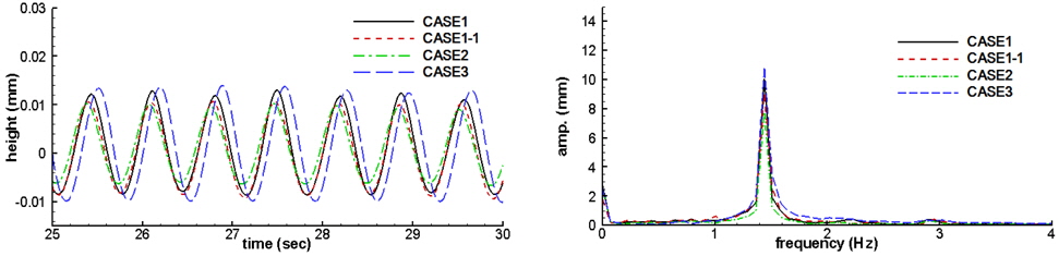
The pressure variation on the lee side affects the height of transmitted waves. The pressure on the lee side of CASE 3 is much higher than those of other cases as shown in Fig. 13. Therefore the transmitted wave of CASE 3 is largest among the cases as shown in Fig. 16. The transmitted waves are measured at x = 0.5m. On the contrary, the transmitted wave height of CASE 2 is smallest among the cases due to the same reason. In CASE 1, CASE 1-1 and CASE 2, the break water moves to right side due to the wave loads. Especially, the horizontal displacement of CASE 2 is larger than any other as shown in Fig. 14. In CASE 3, on the contrary, the breakwater does not move to right side because of the large pressure on the lee side as shown in Fig. 14. Therefore the tension on the mooring line of CASE 3 would be smaller than any other. In contrast the tension on the mooring line of CASE 2 would be largest due to large horizontal displacement.

In the present study, the numerical simulation method developed by Lee and Jeong (2013) was verified for the simulation of two-dimensional floating body and applied to two-dimensional breakwater. To verify the present numerical method, 'lock-in' phenomena on the circular cylinder are simulated and the results are compared to existing research data and the results shows that the present numerical method is applicable to the simulating a translational movement of a body due to fluid force. A few spurious pressure oscillations are occurred but these are ignorable. Free roll decay also simulated. Because the present method cannot resolve the boundary layer accurately in high Reynolds number, there are some differences when the roll angle is larger than 6°. However, when the roll angle is smaller than 6°, the agreements are good enough to apply the present method to the simulation for floating breakwaters.

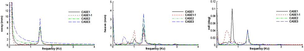
The attenuation performance of a floating breakwater is investigated using the present method. Wave overtopping due to small free board reduces the horizontal displacement of floating breakwater since the pressure on the weather side is reduced. The overtopped water also reduces the heave motion. The high pressure on the lee side of trapezoidal shape (CASE 3) drasticcally reduces the horizontal displacement of floating breakwater; however, the high pressure increases the height of transmitted wave. On the other hand, the small pressure on lee side of the rectangular shape (CASE 2) increases the horizontal displacement but the height of transmitted wave is reduced. Rectangular type floating breakwater has the advantage in calming harbors and trapezoidal shape floating breakwater has the advantage in the small tension on mooring lines.

For more accurate simulation, a method to resolve the boundary layer near the wall has to be developed. Moreover, the present numerical method has to be extended to three-dimension to consider oblique incident waves and the wave deflection.