During ship design, welding-induced distortions are roughly estimated as a function of the size of the component as well as the welding process and residual stresses are assumed to be locally in the range of the yield stress. Existing welding simulation methods are very complex and time-consuming and therefore not applicable to large structures like ships. Simplified methods for the estimation of welding effects were and still are subject of several research projects, but mostly concerning smaller structures. The main goal of this paper is the application of a multi-layer welding simulation to the block joint of a ship structure. When welding block joints, high constraints occur due to the ship structure which are assumed to result in accordingly high residual stresses. Constraints measured during construction were realized in a test plant for small-scale welding specimens in order to investigate their and other effects on the residual stresses. Associated welding simulations were successfully performed with fine-mesh finite element models. Further analyses showed that a courser mesh was also able to reproduce the welding-induced reaction forces and hence the residual stresses after some calibration. Based on the coarse modeling it was possible to perform the welding simulation at a block joint in order to investigate the influence of the resulting residual stresses on the behavior of the real structure, showing quite interesting stress distributions. Finally it is discussed whether smaller and idealized models of definite areas of the block joint can be used to achieve the same results offering possibilities to consider residual stresses in the design process.
The welding simulation is today a wide-spread method to predict the welding-induced distortions and residual stresses. Not the process is modelled here, but the heat-input into the weld.
First attempts to explain the effects of the weld process in a scientific way started with the development of heat conduction models. Already in 1941, Rosenthal (1941) published a set of formulae for the calculation of the temperature field due to a moving heat source. 1952 appeared one of the detailed books by Rykalin (1952) for the calculation of the temperature development during welding. In the 1980’s, these theories were further developed by Lancaster (1986). Different partial phenomena such as the formation of the arc with plasma flux, the vaporization at the surface of the molten weld pool, the melting and dropping of the electrode as well as the forming of the weld bead surface were increasingly included in the investigations (Karlsson and Lindgren, 1990; Lowke et al., 1992; Choo and Szekely, 1994; Hoffmeister, 1986; Ruyter, 1993; Böllinghaus, 1995). Up to then the individual models were only partially combined to models for engineering purposes (Haibach, 2002; Radaj, 2003; Rörup, 2003; Radaj et al., 2006). The accuracy of the simulations was determined in the past mainly by the limited computer capacity. With the increasing development in this area, new possibilities exist to increase the accuracy of the models.
Generally, different levels of accuracy of such simulations exist, starting from the modelling, followed by the implementation of the temperature-dependent material data until the consideration of the phase transformation. The more parameters are considered in the computation, the larger will be the time required for the solution. For this reason, the considered geometry is far idealized in many cases, however, it has been seldom verified up to now if the original geometry behaves in the same way, i.e. the results are comparable and transferable. Therefore, the main objective of the investigation presented here is to develop a method which allows the computation of relatively large geometries. A block joint in the forward part of a RO/RO vessel is considered. Local regions, idealized with small models, are compared with the results of the original geometry (block joint) so that conclusions regarding the comparability and transferability of the results from small models can be drawn and the simplified models can be used during fatigue design. All computations were performed with the finite element program ANSYS.
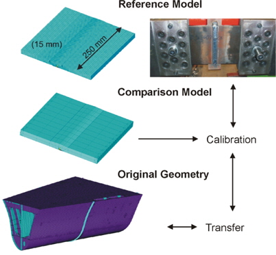
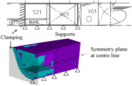
In addition to the computing time mentioned above, another problem exists during the investigation of large structures: The validation of the results is frequently impossible. Therefore it is very important to verify the algorithm chosen. The application of the welding simulation to the block joint considered requires simplifications because otherwise computation times of several months would have to be expected. A stepwise reduction of the mesh density is performed, starting point for the calibration of the different mesh density is a reference model which was thoroughly investigated and validated in an extensive research project (Zacke and Fricke, 2011). As shown in Fig. 1, a comparison model is calibrated against this reference model, the former containing the necessary simplifications in order to transfer the process to the block joint (original geometry).
Higher-tensile ship structural steel D36 was used as material, which can be welded well using a rutile flux-cored wire. The welding process was an automatic metal-active gas (MAG) process, The temperature dependent material data required for the welding simulation were taken from Wichers (2006) assuming no effects from steel grade.
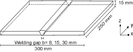
The reference model consists of a plate with a 250
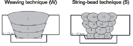
The V-shaped weld was produced using two different welding techniques: The string-bead technique (S) and the weaving technique (W), see Fig. 3. In the research project (Zacke and Fricke, 2011), also the effect of the gap width was investigated, which is not further described here.
Blocks are frequently joined by the weaving technique owing to simpler handling. Rules (VSM, 2006) require a max. gap width of 25

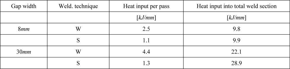
Heat input.
Due to the different number of beads per layer, the first impression is that the weaving technique introduces twice the energy of the string-bead technique into the weld. This value is used for the welding simulation of the reference model (heat input per bead), as each string-bead is simulated. In the simplified models, the heat input into the whole weld section is used as only one layer could have been implemented to limit the computing time.
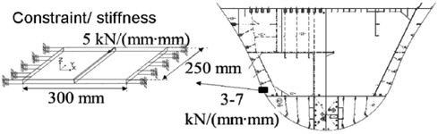
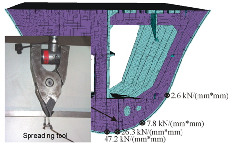
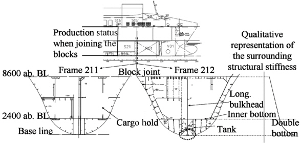
The plate of the reference model represents only a section of the block joint, therefore the stiffness of the surrounding ship structure needs to be taken into account by the boundary conditions at the plate edges parallel to the weld. In order to determine this stiffness, measurements were performed with a spreading tool at the block joint before welding the shell plate (Huismann and Savu, 2001), see Fig. 4.
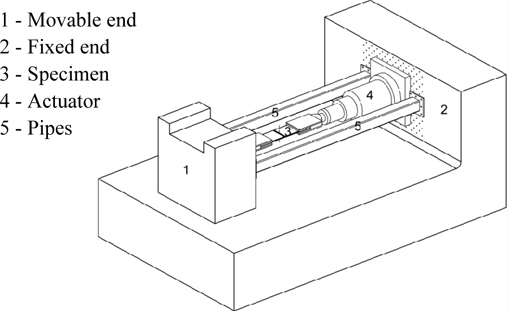
From the measurements, a typical stiffness just above the inner bottom was selected and realised in a restraining welding set-up, see Fig. 5. A closed force loop was provided, using two pipes connecting the fixed and the movable ends. The pipe dimensions determine the stiffness of the system.
The reaction forces transverse to the weld during and after welding, which are an important part to validate the welding simulation results, were measured by the load cell in the actuator, which kept a constant displacement at the fixed end. Both welding techniques were applied and simulated, however, only the weaving technique used for the calibration is shown here. Fig. 6 shows the numerical model which is characterized by a high mesh density. The path of the heat source follows that of the welding nozzle as illustrated in the figure.
Along this path, the transient heat source according to Goldak et al. (1984) has been used, applying the heat flux densities to the nodal points. All necessary welding parameters correspond to those during the experiment where also the weld pool dimensions were recorded to be used for defining the heat source.
The thermal analysis is followed by a structural analysis, using the temperatures determined in the first analysis as loading in order to compute the strains. The resulting residual stress and deformation state serves as reference and is the basis for calibrating the comparison model. The results are discussed by Zacke and Fricke (2011) in detail and will be presented together with the other models below.
A great number of approaches exist to simplify the algorithm for calculating residual stresses. The objective of the calculation has to be taken into account and determines or limits admissible measures; therefore, these have to be defined at first: the residual stress state of the original geometry (block joint) shall be determined. It is not wanted to compute the exact residual stress distribution in the local weld region where very high temperature and stress gradients occur which would require a very fine mesh. This local area is restricted to about 2.5 times the weld seam width acc. to Osawa et al. (2007).
Furthermore, it is assumed that phase transformation and the associated changes in material data do not have a significant effect on the development of residual stresses. The effects of phase transformation are, of course, known and can be considered in specialized simulation software, however, the welding simulations of the reference model (Zacke and Fricke, 2011) have shown that the distortions and the reaction forces can be well determined when neglecting phase transformation.
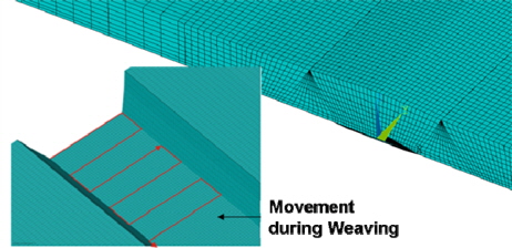
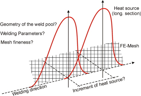
Apart from the knowledge of the input parameters, decisive is the necessary mesh fineness when performing a welding simulation. Normally, element lengths of a few millimetres are used which lead to an enormous number of nodal points. The requirement of small elements is due to the high temperature gradients. If these are not correctly reproduced, the resulting strains and stresses and also the reaction forces cannot correspond to reality. Therefore, the temperature field with its input parameters and mesh density are calibrated with measurements. The temperature distribution is created by a heat source which represents the welding nozzle respectively the feed wire at a definite instant of time. As the nozzle is moving continuously along the weld, the question has to be answered how the increments of the heat source are defined during the simulation. Fig. 7 illustrates the situation.
From an engineering point of view, the essential problem is the correct heat input of the total energy and the formation of the three temperature gradients in space. As the focus is only on global residual stresses, it seems to be logical to calibrate the model on the basis of the measured reaction forces which result from the shrinking due to the thermal load. This has the advantage that a coarser mesh is possible as the final stage is compared and not the temperature field resulting from the first step of the analysis.
These considerations are necessary as the finite element model has a large number of nodes in any case so that a factor of e.g. two has a tremendous effect on the computation time. The calibration on the basis of reaction forces now allows the following simplifications:
• Reduction of the multi-pass to a single-pass weld • Increase of the element length (and hence, the increment of the heat source)
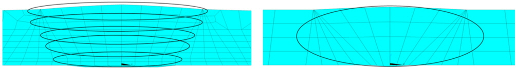
Fig. 8 shows the simplifications in the comparison model (one pass) compared to the reference model (five passes). The total heat input determined from the welding specimens was kept the same. Furthermore, the weld pool dimensions have to be adapted for the single-pass weld, otherwise the actual temperature would not be realised in all locations of the weld. The chosen weld pool dimensions are indicated in Fig. 8.
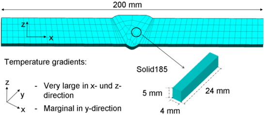
Regarding the element sizes, the dimensions shown in Fig. 9 were chosen for the 200
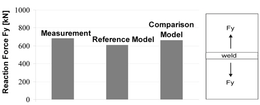
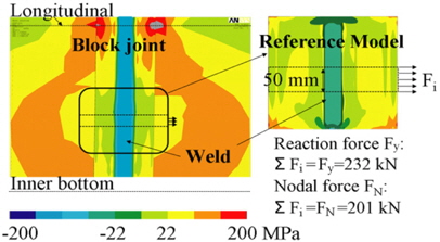
The calibration with respect to the reaction forces is performed with the welding parameters used for the comparison model. Fig. 10 shows a comparison of the reaction forces Fy measured after cooling and computed with the reference and comparison model. The results confirm that the chosen simplifications are possible without changing significantly the energy input. Stresses will be compared in connection with results obtained for the original geometry (block joint).
ORIGINAL GEOMETRY (BLOCK JOINT)
The original geometry is a block joint in the forebody of a 193
The finite element model of the blocks consists of shell elements. However, the simulation of the welding process requires solid elements because it can result in high gradients in all three directions concerning the heat flux, the temperature as well as the stress and strain distribution. A multi-layer shell structure could also model this, however, as the comparison model has already shown satisfying results, the original geometry is modelled at the joint in the same way.
Here, a 200
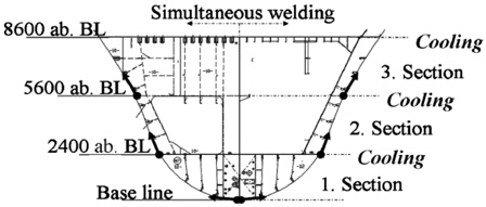
Welding sequence has been defined according to the standards of the shipyard Flensburger Schiffbau-Gesellschaft. Starting point is the center of the base line. From there, welding is performed with the weaving technique by a Bug-O-Mat automatically in three sections upwards, see Fig. 12. Both ship sides are welded as far as possible simultaneously, hence, a half model with symmetry conditions is used in the following. After welding each section, a cooling phase follows during which the guide rails are relocated.
The other boundary conditions are illustrated in Fig. 13: A fixed end has been assumed aft where the blocks are already connected to the blocks behind. Simple supports are arranged along the center line below the bottom, where elastic spring stiffness of the wooden blocks was neglected. It has been checked during calculation that no lifting forces occur at the supports.
VALIDATION OF THE SIMPLIFICATIONS
The procedure is validated by comparing the results of the original geometry (block joint) with those obtained for the comparison model containing the same simplifications and the reference model for which extensive measurements have been performed. These are the basis for the validation, see also Fig. 1.
As illustrated in Fig. 14, the reference model, which represents a section of the block joint due to its constraining conditions, corresponds to a section in the first plate field just above the inner bottom. The calculated residual stresses are compared with those in the reference model in the following.
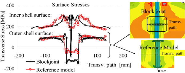
Fig. 15 shows this comparison. The plots display the stresses on the shell surface transverse to the weld. Both plots show tensile stresses in the weld region which turn into compressive stresses in a distance of about 30
The surface stress distribution is further evaluated in Fig. 16. Here, the stress distribution along a path transverse to the weld is plotted for the outer and the inner shell surface, i.e. showing bending effects. On the inner surface, tensile stresses of about 200
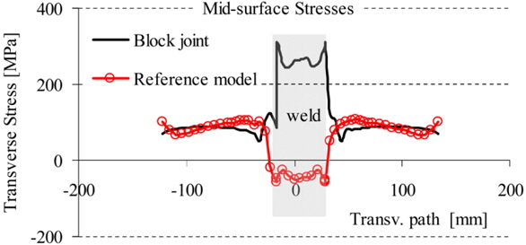
The same observations can be made for the mid-surface stress, see Fig. 17. These amount to about 100
The distribution of the transverse residual stresses depends mainly of the shrinkage forces and the resulting deformations. The welding simulation for the block joint was simply performed only with one pass, and the highest tensile stresses occur in the weld approximately at the location of the heat source. This was assumed at about 3/4 height of the plate thickness resulting in bending deformations agreeing well between the reference and comparison model. Therefore, the total shrinkage force and the bending effects are well taken into account, but the distribution of the shrinkage forces over the plate thickness is not correctly considered. This effect occurs only locally in the weld and decays already 20-30
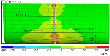
The welding simulation was performed as shown in Fig. 12 in three sections. The computation time of clustered workstations was six days. The results presented in the following refer only to longitudinal membrane stresses in the components. Fig. 18 shows these stresses in the shell after the weld in the third section has cooled down. The stresses represent the global stress state acting transverse to the weld line.
The first impression is that the welding of the block joint affects a large region when looking at the resulting residual stresses. The longitudinal stresses reach values between 11 and 33
A high stiffness is present in the lower part of the double bottom, i.e. in way of the center line, which is due to the longitudinal bulkhead and the center line girder. The residual stresses are locally larger than 200
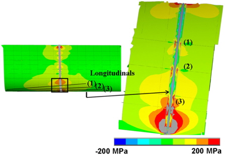
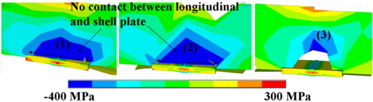
The high stiffness at the longitudinals is due to the fact that these are already connected when the shell plates are welded, resulting in high longitudinal stresses. For equilibrium reasons, a high compressive stress must be present in the longitudinals. Fig. 20 shows the longitudinals at the intersection points (1)-(3). Above the block joint, which can be recognized by the solid modelling, a horizontal slit is arranged at the intersection points (1) and (2), i.e. there is no connection between the components over a length of 200
The intersection points (1) and (2) show very high compressive stresses in the longitudinals above the slit which is due to the high stiffness there. At point (3), a reduced area of high compressive stresses is observed. The main reason for the differences are the different shape and length of the non-welded part. A significant effect on the residual stresses in the shell plate cannot be seen. The shrinkage force creates additional bending of the longitudinals with tensile stresses at their top.
In accordance with Fig. 17, high tensile stresses can be seen in the center of the weld, which decay with increasing distance from the weld.
In summary it is stated that critical areas with high tensile stresses exist in the shell plate at points with high stiffness. These are in particular the intersection points with the longitudinal components. At longitudinals, stresses of up to 200
The paper describes the application of the numerical welding simulation to a block joint in shipbuilding. The main objective is the determination of the residual stresses occurring due to the constraint by the surrounding structure. Its effect was at first studied by 250
As numerical welding simulation requires a very fine finite element mesh to consider steep gradients in temperature and strain, it can currently be applied only to relatively short welds and not to long welds like those of block joints in shipbuilding. However, the objective of determining global residual stresses allows some simplifications of the models which were validated by a comparison model against the fine-meshed reference model representing the specimen with 250
The simplifications allowed the numerical welding simulation of the whole block joint to be performed. The distribution of the residual stresses was strongly influenced by areas of high stiffness, e.g. at the longitudinals and girders, where global tensile residual stresses occur which remain below the yield stress. The agreement with the overall stresses in the reference model was quite good in the areas where the stiffness was the same as in the constraining welding set-up.
In a conclusion it is proven that substantial simplifications are possible if the numerical welding simulation of block joints is only aimed at the overall residual stresses and distortions. On the other hand, the computation of the reference and comparison models for the 250