In this paper, an iterative boundary element method (IBEM) was proposed to solve for a wing-in-ground (WIG) effect. IBEM is a fast and accurate method used in many different fields of engineering and in this work; it is applied to a fluid flow problem assessing a wing in ground proximity. The theory and the developed code are validated first with other methods and the obtained results with the proposed method are found to be encouraging. Then, time consumptions of the direct and iterative methods were contrasted to evaluate the efficiency of IBEM. It is found out that IBEM dominates direct BEM in terms of time consumption in all trials. The iterative method seems very useful for quick assessment of a wing in ground proximity condition. After all, a NACA6409 wing section in ground vicinity is solved with IBEM to evaluate the WIG effect.
h Clearance of the wing from the ground AoA Angle of attack ε Pre-described error for the IBEM analyses c Chord length of the wing N Number of discretized panels
Effect of the ground has several impacts on a structure flying above the surface. These structures use the several benefits that the surface serves to them, which is named as ground effect flight. Different definitions of ground effect can be found in the literature and one of them defines it as “a phenomenon of aerodynamic, aeroelastic and aeroacoustic impacts on platforms flying in close proximity to an underlying surface” (Reeves, 1993; Rozhdestvensky, 2006). Efficient utilization of the ground effect proposed a different transportation technique other than mainly used, when the Russians first made use of it during the cold war (Rozhdestvensky, 2006).
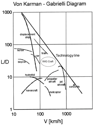
Although first built for militaristic purposes, ground effect is a phenomenon that is generally exploited by Wing-in-Ground (WIG) effect crafts to improve transportation efficiency. Analyzing the Von Karman-Gabrielli Diagram (see Fig. 1), WIG vehicles fill the gap between very efficient but slow conventional ships and not that efficient but very fast airplanes.
WIG crafts can be a good alternative for transport over the sea due to their lower fuel consumption. They spend less fuel than hydrofoil vessels and hovercrafts which are also accepted to be high speed marine vehicles like WIG crafts. The closeness of WIG crafts to the technology line assures these vehicles’ availability to be widely used.
Up to now, these vehicles have not been built and exploited from their advantages due to a few reasons. On behalf of stability problems and some safety issues, there is still some way to go to improve their efficiency. The efficiency of a wing is determined by the lift-drag ratio and these parameters may either be calculated numerically or experimentally. There are many works on wing-in-ground effect and a large part of these works focus on the augmentation of lift and reduction of drag that the ground creates over the wing. An optimal design with the goal to achieve maximum lift satisfying the height stability criteria of a WIG craft was developed by Kim et al. (2009). They have assumed inviscid flow and used vortex lattice method to optimize WIG by sequential quadratic programming. Wing configurations on a wing-in-ground effect in terms of efficiency were investtigated by Lee et al. (2010). Djavareshkian et al. (2010) have investigated the effects of a smart flap under ground effect and proved an increase in efficiency by CFD. Ahmed and Sharma (2005) analyzed a symmetrical NACA0015 wing section experimentally and concluded their work with the optimum conditions for maximum lift and minimum drag. Evaluation of a power augmented ram (PAR) as a lift booster in take-off and landing was made by Zhigang and Wei (2010). Flow around a WIG craft with and without PAR was analyzed by CFD in their work.
Although WIG analyses are generally made with commercial softwares that use RANSE such as (Abramowski, 2007; Jamei et al., 2012), potential flow codes are also frequently used to assess a wing-in-ground effect. Other than the work of Kim et al. (2009), lifting surface theory which adopts the inviscid flow assumption was used in numerous works by Liang and Zong (2011), Zong et al. (2012) and Liang et al. (2013). Phillips and Hunsaker (2013) have used potential based lifting line theory to assess the closed-form relations that were offered to assess the effect of the ground over the wing sections. Some benchmark experimental studies are found in the literature as well, like Luo and Chen’s (2012) work on NACA0015 wing or the work of Jung et al. (2008) on NACA6409 wing. Daichin (2007) analyzed the near-wake flow of a NACA0012 airfoil above a free surface experimentally with PIV. It is concluded in his study that as the clearance from the free surface decreases, the wake flow of the airfoil remarkably changes.
WIG crafts may have complex geometries and solution of the flow around these bodies may be time consuming using RANSE. Construction of the mesh system and to produce a result takes relatively greater times. Due to this reason, many potential theory based articles implement the boundary element method as a numerical approach. Boundary element methods panelize the objects inside the fluid rather than meshing the whole fluid domain to calculate the flow characteristics around them. The number of objects in the fluid does not matter; as there may be single or multiple object(s) inside the fluid. Direct application of boundary element methods enables solving the whole flow even if there are many objects inside the fluid. However, a different treatment of the method that leads to the solution iteratively produces faster results. In this article, an iterative boundary element method (IBEM) will be used to solve the two-dimensional fluid flow around a wing in ground proximity. The existence of a ground underneath a wing makes up the case of multiple objects inside the fluid; and with boundary element method, this problem can be solved via an iterative approach.
Incompressible and inviscid continuity equation for an irrotational fluid is defined by the Laplace Equation which states that the total potential

According to the Green’s Identity, a general solution of the Laplace Equation can be given as a sum of source and doublet distributions on the boundary of a 2-D surface S. This is defined in Eq. (2):

In this equation,

Neumann boundary condition states that there is zero normal velocity on the body surface which can be written as:

In this work, Dirichlet type boundary condition is used; therefore, in terms of the velocity potential, direct boundary condition transforms into the indirect boundary condition:

If the indirect boundary condition is applied to the Green Theorem, Eq. (6) is obtained for the Dirichlet type of boundary condition:

Internal velocity potential is selected to be equal to the free-stream velocity potential, therefore Eq. (7) which is derived from Eq. (6) becomes:

Rearranging the Neumann boundary condition leads to:

The derivative of the perturbation potential becomes equal to the negative of the normal free-stream velocity. This boundary condition is given by Eq. (9):

Setting the value for the discontinuity in the normal derivative of the velocity potential to source strength, and keeping in mind that internal velocity potential is equal to zero due to:

The only unknown in Eq. (7) is now the dipole source strengths
It is possible to divide an arbitrary surface S into N panels to construct a numerical solution following Green’s identity with Dirichlet type of boundary condition given in Eq. (6). If Eq. (6) is to be performed for each panel of the surface (and the wake), we may write:

To reduce into a more compact form, it is accepted that:


Substituting the values of Eqs. (12) and (13) into Eq. (11) and setting the constant equal to


Applying the Neumann boundary condition:

Examining Eq. (14), it may be observed that the only unknown in the equation becomes the doublet strengths
After the derivation of doublet strengths, potential and velocities at each point inside the flow can be found by finite difference method.
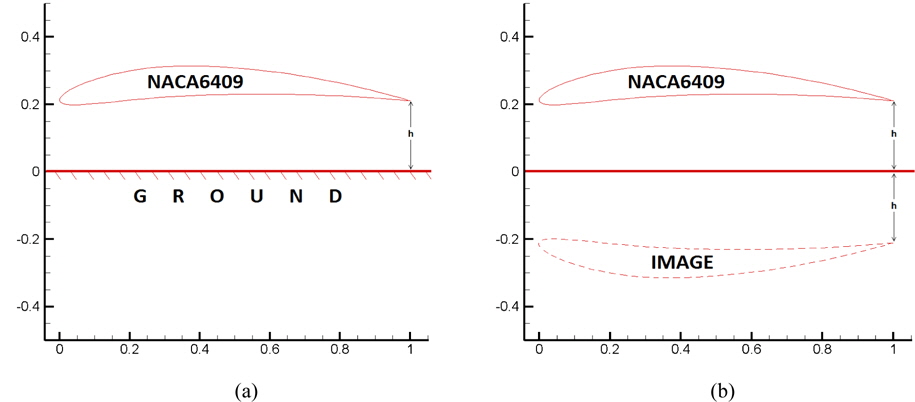
Ground may be represented by the image method as a numerical approximation to the real case. Image method states that if a ground is present underneath an object inside the flow, the effect of the ground can be calculated by taking into account the image of the real object (Katz and Plotkin, 1991). Please refer to Fig. 2 for a better presentation. In that Figure, a NACA6409 wing with 0° angle of attack is in ground proximity.
In this study, method of images was implemented to both direct and iterative boundary element methods for the representation of the ground effect. It is accepted that ground effect in this article covers land only. WIG crafts can also operate over water, however; due to approximately 1/800 density ratio of the air to the water, the water behaves like land in this situation. There may be a small decrease in the lift when operating over water but this is of small importance and can be neglected. To understand the effects of the free water surface to a wing-in-ground effect, please refer to Liang and Zong (2011) and Zong et al. (2012). To comprehend the free surface deformation at high Froude numbers for a wing-in-ground effect, please see Barber’s numerical work (Barber, 2007).
>
Direct boundary element method
The geometries inside the flow will be divided into panels and in each panel, there will be collocation points at which all the calculations will be made. On each collocation point, constant strength sources and constant strength doublets will be distributed and at all these collocation points Eq. (14) must be satisfied. Let’s say a body inside the fluid has
>
Iterative boundary element method
When objects in the flow have complex shapes and must be represented by large amounts of panels, the sufficiency of a computer may be questioned. For example, if
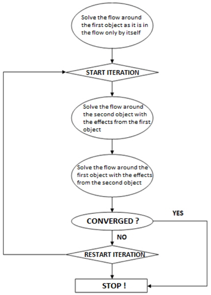
An alternative method is the iterative boundary element method which suggests solving the problem separately. In the iterative approach, the problem is broken into parts to solve for each part separately; and then is reunited to go for a final solution.
With this approach, the real wing which is in ground proximity is solved first as if it is inside an unbounded fluid. The doublet strengths and the induced potentials by the wing in the outer flow are calculated. Then, the image wing is solved as if it is inside an unbounded fluid. However this time, off-body potentials induced by the real wing are added to the potentials induced by the image wing to integrate the effects of the interaction of the real wing with the ground. What is done here is the superposition of the flow around the image wing in an unbounded fluid with the effects induced by the real wing. After this step, attention turns to the real wing. Off-body potentials induced by the image wing on the real wing are added to the flow around the real wing in unbounded fluid. With this step, the effect of ground proximity is reflected to the real wing. Here;

Iterative boundary element method has a wide range of applicability from electromagnetism to heat transfer. It is also used for fluid flow problems as Bal (Bal,2003; Bal,2007; Bal,2008; Bal,2011) has selected works on the topic. However; the emergence and widely usage of the IBEM dates back to 1990’s when Lesnic et al. (1997) have proposed the method for the solution of the Cauchy problem for the Laplace equation, Up to now, IBEM has been used in many different fields and proved its worth in time.
>
Validation with the single case
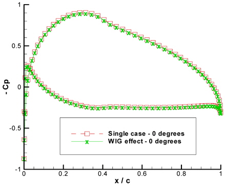
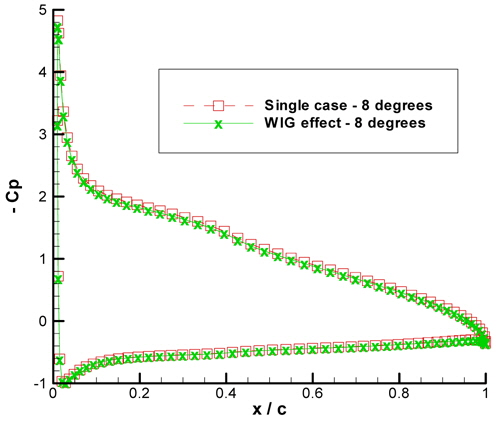
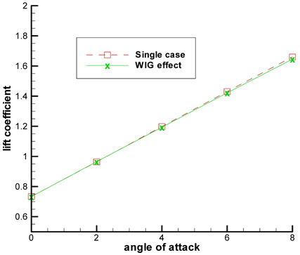
A wing in ground effect loses its advantage as it moves away from the ground. At infinite clearance, the wing will act like as if it is inside an unbounded fluid. If the ground is adequately far enough from the hydrofoil, then we must expect the hydrofoil to have its naked lift (as if there was nothing affecting the flow of the hydrofoil). To validate the results, a wing section of NACA6409 was chosen with the ground clearance selected to be
The lift coefficients obtained at various angle of attacks for 10×

[Table 1] Lift coefficients obtained for WIG effect and the single case.
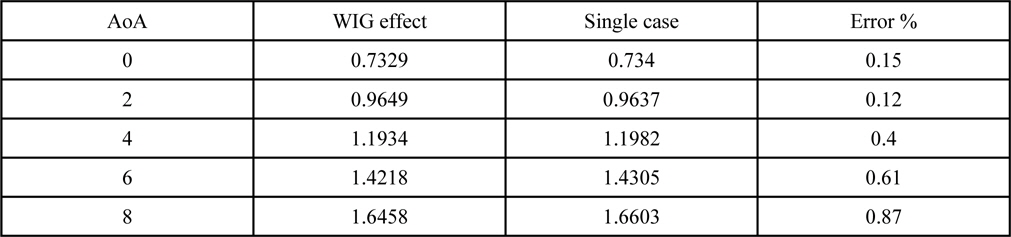
Lift coefficients obtained for WIG effect and the single case.
Table 1 points out the precision the IBEM produces as the maximum error generated is less than 1%. The graphical view of table 1 is given in Figs. 4-Figs. 6 shows the negative pressure coefficient distribution for 0° and 8° of angle of attack obtained both ways respectively.
>
Validation with direct BEM and CFD
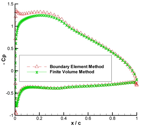
As a first step, results derived with the boundary element and the Finite Volume Methods (FVM) were compared for a single NACA6409 with an angle of attack of 4° in an unbounded fluid. Due to the absence of the ground effect, direct BEM was used. Obtained lift coefficient values were in good agreement as BEM found 1.1982 while FVM found 1.1857 for the wing. Fig. 7 shows the negative pressure coefficient distribution derived with BEM and CFD. Except the leading edge region of the suction side, both methods gave compatible results with each other.
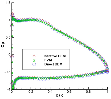
To prove the effectiveness of the IBEM, the obtained results are compared with the results obtained with Direct BEM and CFD. This time, the same wing section was solved with ground clearance
Analyzing Fig. 8 will lead to the conclusion that IBEM is as strong as Direct BEM as the values found with both methods overlap. Overall, IBEM shows up to be a good alternative to Direct BEM and FVM.
>
Validation with results from the literature
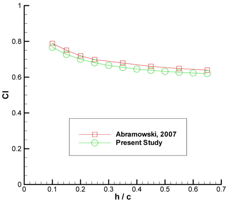
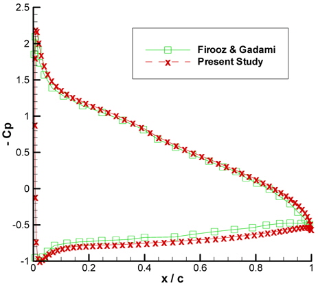
Up to now, results found with IBEM seems to be in good agreement with the other methods. At this part of the paper, the results produced with the iterative method will be compared with the results found in the literature. This will be done in two steps. First, the lift coefficients produced with IBEM will be compared with Abramowski’s (2007) work and then the pressure distribution will be compared with the results produced by Firooz and Gadami (2006).
Abramowski (2007) have investigated the ground effect over a NACA/Munk M15 airfoil. Lift coefficients at different ground clearances have been found. Results found with IBEM is compared with the results in that study and this is given in Fig. 9.
Although the results produced by IBEM is slightly lesser than Abramowski’s (2007) results, they pretty seem to be in accordance. Pressure coefficient distribution along a NACA4412 airfoil is compared with Firooz and Gadami’s (2006) work. Fig. 10 exhibits this comparison and the results are again compatible.
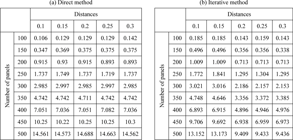
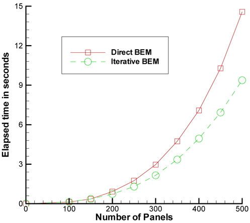
Applicability of the iterative method relies on the results of time consumption. Iterative boundary element method will be preferred in problems containing high number of panels which will give solutions slower. IBEM stores fewer values in the computer’s memory while the direct boundary element uses more computer memory. This difference between the stored values of both methods leads to differences in the acquisition of a solution. IBEM responds more quickly and gives faster results (Kinaci et al., 2011).
To fully comprehend the advantage IBEM offers, a test case of a two dimensional NACA6409 wing with 0° AoA in ground effect was solved in different clearances from the ground for various numbers of panels. The results of the test case are given in Table 2.
Distances in Table 2 are dimensionless and given in

Time elapsed in seconds for direct (a) and iterative methods (b). Number of panels is listed vertically while distances are listed horizontally in these tables.
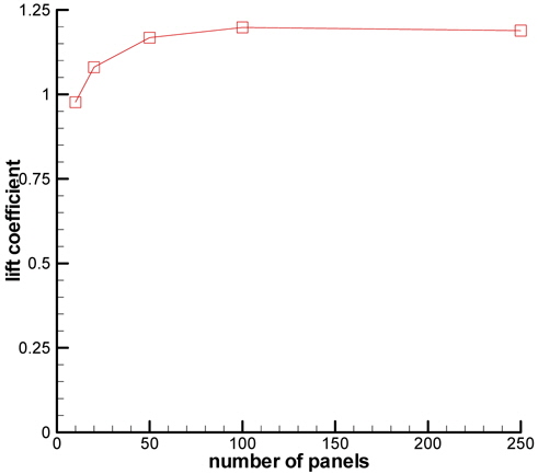
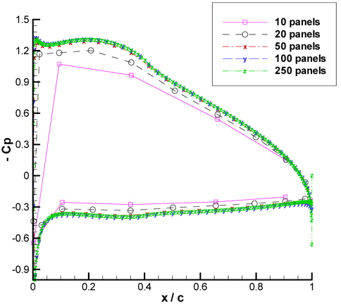
Grid dependency is investigated by single precision BEM for a single NACA6409 wing at 4° of AoA. The lift coefficient and the pressure coefficient distribution along the wing is examined for 10, 20, 50, 100 and 250 panels. The lift coefficient vs. number of panels is given in Fig. 12.
The lift coefficient seems to be converging as the number of panels increase; changing from about 0.95 for 10 panels to about 1.2 for 100 panels. However; it must be noted that there is a slight decrease in this value when the number of panels is 250. Therefore, the pressure coefficient is also closely observed to inspect possible errors in the distribution. Fig. 13 exhibits the pressure coefficient distribution along NACA6409 wing.
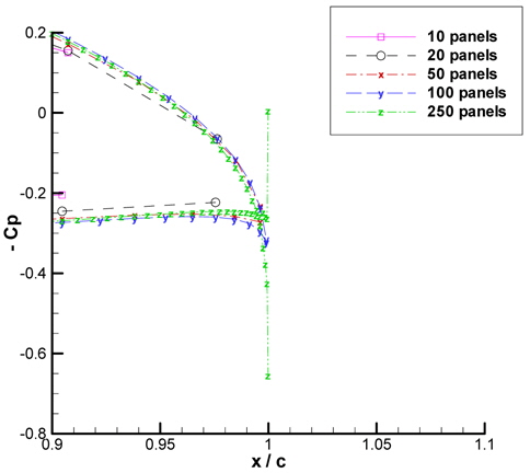
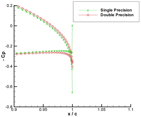
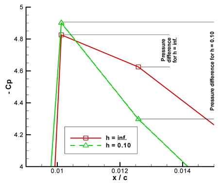
It is derived from Fig. 13 that as the number of panels increase, the pressure coefficient distribution along the wing converges. However for 250 panels, it seems from Fig. 13 that the Kutta condition is violated; the velocity at the trailing edge does not seem to be zero. Please see Fig. 14 for a closer view at the trailing edge.
As the number of panels increase, the size of each panels decrease; leading to very small values of panel distances for the wing. So it is hypothesized that the precision of the solver must be increased to truly represent smaller panels. It can be derived from Fig. 15 that this hypothesis is in fact true because the Kutta condition seems to be satisfied with double precision solution.
If the single precision BEM is used, 100 panels seem sufficient to discretize the geometry. Greater number of panels leads to smaller sized panels which the single precision solver cannot perceive. It is found out that for double precision BEM, the number of panels for the wing can go up to 250 panels. Kutta condition will correctly be represented as the precision of the solver increases for increasing number of panels.
GROUND EFFECT ON A NACA6409 WING
Up to this point, the accuracy and the efficiency of IBEM was proved. The code developed with the theory of IBEM was then used to assess a two dimensional NACA6409 wing-in-ground effect. Extreme ground effect (which is when the wing is
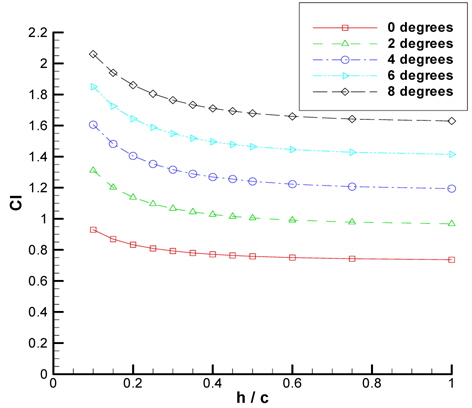
The calculations are made for five different AoA values which are 0°, 2°, 4°, 6° and 8°. The solver is set to single precision, discretizing each wing with 100 panels. The change in lift coefficient at different AoA values is given in Fig. 16 The wing creates more lift as it gets closer to the ground. As the AoA of the wing increases, the wing shows tendency to create more lift in lower ground clearances. The curves get steeper as the AoA increases. Please see Fig. 16 for a better view.
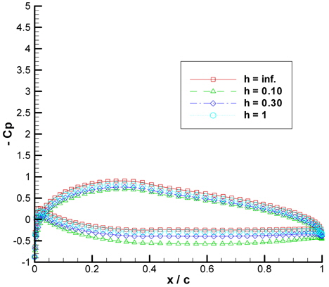
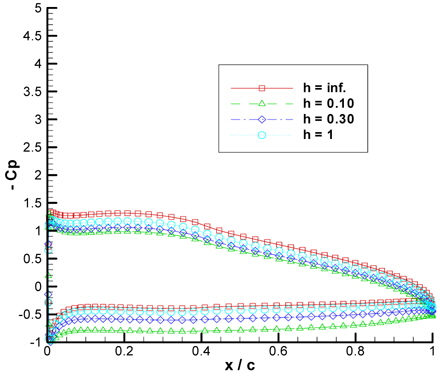
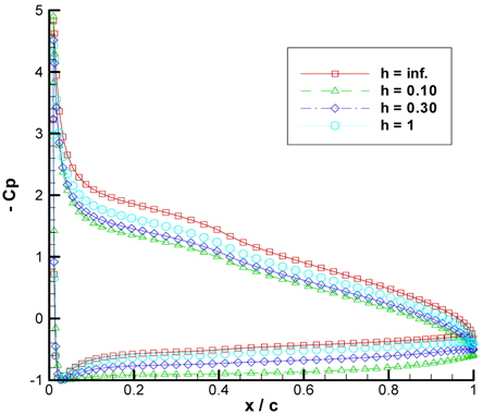
Negative pressure coefficient distributions along the NACA6409 wing in different ground clearances are given in Figs. 17, Figs.18 and Figs.19 for 0°, 4° and 8° of AoA respectively.
In Figs. 17-Figs. 19; the difference between the suction and the pressure side of the wing increases as the wing has higher AoA which explains the reason of higher lift. The pressure coefficient distribution tends to get closer to the condition of unbounded fluid (which is the case of
The increase in AoA sharply leads to an increase in the flow velocity at the leading edge. Ground proximity for a wing also plays a role in the rise of fluid velocity at this part of the wing. Although viscous forces are not included in this study, this explains the flow separation incident. When there is a big difference in velocities (or pressures) at two neighbor points on a body, the flow cannot follow the body surface and separates. Vortex motions may be formed which will lead the case to unsteady flow and an unstable condition for the wing. Therefore; stall may show up earlier in ground proximity and this phenolmenon must especially be avoided in WIG crafts. Stall of the wing will cause the craft to oscillate causing danger and discomfort for the passengers. Please refer to Fig. 20.
For high AoA conditions of the wing in closer ground proximities, it is suggested that unsteady IBEM to be used to detect oscillations and vortex formations around the wing. This way, the lift and the pressure around the wing can be retained more precisely.
In this paper, an iterative boundary element method for a solution of the flow around a wing-in-ground effect was proposed. Compared to RANSE solutions BEM is quite faster; which only discretizes the body inside the fluid rather than the whole fluid domain. However, as shown in this paper, there are methods to increase the efficiency of BEM. Iterative BEM is faster and has good precision, therefore; it seems to be more efficient than direct BEM. Iterative method shows good prospect in dealing with geometries in ground proximity where a higher number of panels must be used. These may include complex bodies of three dimensions in which case the panels will no longer be represented by lines but surfaces which will increase the calculation time significantly. Quick assessment of the efficiency of a particular type of wing section for WIG crafts can be made with IBEM.
When the wing is in extreme ground effect, the wing will possibly oscillate in the air due to vortex separations from the body. This will create unsteady motions for the wing. Unsteady motions will lead the WIG problem to be solved at each time step increasing the necessity for quicker solutions. It is thought that IBEM will prove its real worth in unsteady cases where the solution time is expected to drop significantly. As a future work, the generated code will be developed for solving unsteady motions to include extreme ground effect cases.