The increasing global economy and limitations of fossil fuel availability have encouraged research on renewable energy. Tidal energy is regular, predictable, and available at higher power densities as compared to other weather-dependent renewable resources. Just as in England or Canada, Korea, a leading country of tidal energy generation, has large the resources of tidal energy and has attempted to extract energy with tidal barrages as well as tidal stream generators. An in-situ experiment involving a tidal stream power plant with a helical-bladed Darrieus turbine was carried out at the Uldolmok narrow channel between Jindo islands and Haenam in Korea (Han et al., 2009). However, due to economic and social challenges, the commercialization of hydrokinetic tidal power extraction is not yet realized.

There are several types of tidal stream generators, including drag- or lift-type devices as well as horizontal or vertical axis turbines. A Savonius vertical axis turbine is a typical example of a drag-type device, which usually operates at low speeds. The optimal power coefficient normally occurs when the TSR is lower than 1. There have been many attempts to optimize the power coefficient through parameter studies; however, the maximum recorded power coefficient of the Savonius turbine was found to be nearly 20% (Akwa et al., 2012; Menet and Bourabaa, 2004). Meanwhile, the horizontal-axis turbine (HAT) is known as the most efficient tidal stream generator. In a lab-scale experimental study, the power coefficient achieved was as high as 48% (Batten et al., 2007). In order to achieve high efficiency, the HAT needs to be aligned properly with variable stream lines. In comparison, a Darrieus vertical-axis turbine (VAT) can operate in all flow directions, though it tends to exhibit somewhat lower efficiency than HAT. In an experimental study with a free stream velocity of 1.2m/s, the maximum efficiency was 33% with a straight-bladed Darrieus turbine (Shiono et al., 2002). A helical-bladed Darrieus turbine achieved a power coefficient of 41.2% in an optimal design study (Yang and Shu, 2012).

The computational fluid dynamics (CFD) simulation is frequently used as a numerical approach as an alternate to more expensive experimental studies in order to validate the performances of turbines. Additionally, the blade element momentum theory (BEMT) is a theoretical method that is used for the analysis and design of HATs (Batten et al., 2008; Clarke et al., 2007), with the results showing good agreement with those of lab-scale experiments in terms of the power coefficients. On the other hand, even if the computational cost is high, research using CFD simulations is conducted through three-dimensional analyses of HATs (Lee et al., 2012), as this is a viable means of investigating vortex activities over the surfaces or near the tips of the blades in detail. Meanwhile, for the Darrieus VAT, no current theoretical method perfectly captures its actual performance as compared to detailed CFD simulations (Dai et al., 2011; Islam et al., 2008; Jung et al., 2009). BEMT methods with single- or multiple-stream tube, vortex, and cascades models show improvements in how well they predict the performance of a Darrieus VAT; however, they still exhibits drawbacks. Thus, a CFD simulation becomes a popular tool when used to analyze the performance of a Darrieus VAT (Carrigan et al., 2012; Ghatage and Joshi, 2011; Sabaeifard et al., 2012). Two-dimensional CFD with less computation than three-dimensional CFD is used in the design of sections of Darrieus VATs instead of a theoretical method. For instance, with help of CFD tools, the cambered airfoil was found to improve the self-starting capability of a Darrieus VAT (Beri and Yao, 2011). An increase in the number of blades was also proposed to reduce both the torque and RPM fluctuations (Castelli et al., 2012). Among these approaches for performance improvements, a helical-bladed Darrieus turbine is considered to be a strong candidate for overcoming the disadvantages of a straight-bladed Darrieus turbine, such as the fluctuation of the torque and the RPM as well as the low self-starting capability (Shiono et al., 2002). In order to design the helical-bladed turbine and explore three-dimensional effects such as tip loss, three-dimensional CFD with a high computational cost is mandatory.

The approaches described above involving the use of CFD simulations and the BEMT are typically utilized when the TSR is determined. However, in the actual operating conditions of an experiment, tidal stream turbines begin to rotate from zero angular velocity when the flow speed reaches a sufficient value to rotate them. Afterwards, the TSR of a turbine is determined when a certain load is applied to a turbine in the direction opposite the rotation direction (Bahaj et al., 2007). Although the flow speed is stable under real operating conditions, the TSR as well as the torque are known to fluctuate in Darrieus turbines. Therefore, to capture realistic operational characteristics in an experimental study, a flow-driven rotor simulation, in which the body is driven by the flow, is more appropriate than a simulation with a given TSR. In this work, we introduce a flow-driven rotor simulation using FLUENT with a six-DOF solver to estimate the performance of a Darrieus VAT. First, a three-bladed turbine with the NACA 0020 section, as used in a previous study, is studied in order to investigate its basic performance characteristics in 2D CFD simulations. The performance of a helical-bladed turbine is then investigated as compared to a straightbladed turbine by 3D CFD flow-driven rotor simulations to assess the fluctuation and self-starting capability as well as the power coefficient.

We exploit ANSYS FLUENT, which uses the finite volume method to solve the Navier-Stokes equation as a flow solver. A pressure-based Reynolds-averaged Navier-Stokes (RANS) model is used to compute the flow properties in the unsteady condition. The sliding mesh method is used to transfer fluid media from the inner rotating domain, which contains the turbine, to the outer domain. The shear stress transport (SST) k-ω turbulent model is chosen because it combines the advantage of the k-ω model near the wall and the k-ε model away from the wall. SST k-ω provides superior results for a flow with a strong adverse gradient and separation in turbine simulations (Dai et al., 2010). A second-order accurate model and a second-order upwind model are selected for pressure discretization and momentum, respectively. A second-order implicit transient formulation is used as well. The residual for the convergence check is set to 10-4 in order to obtain an accurate solution.

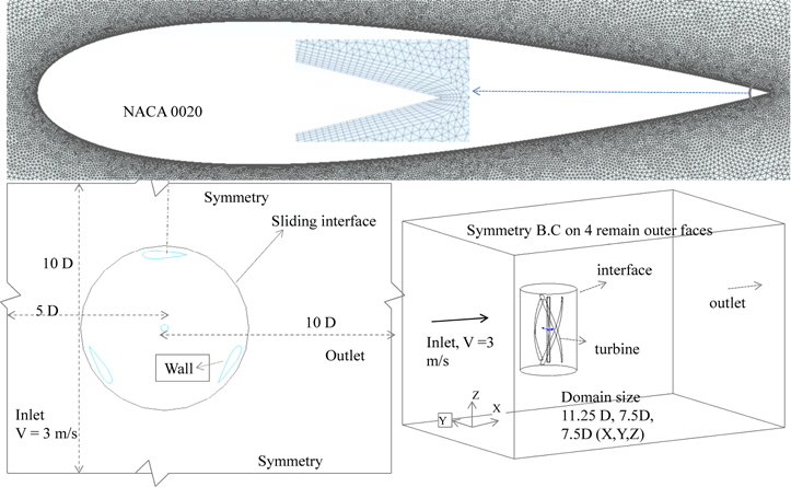
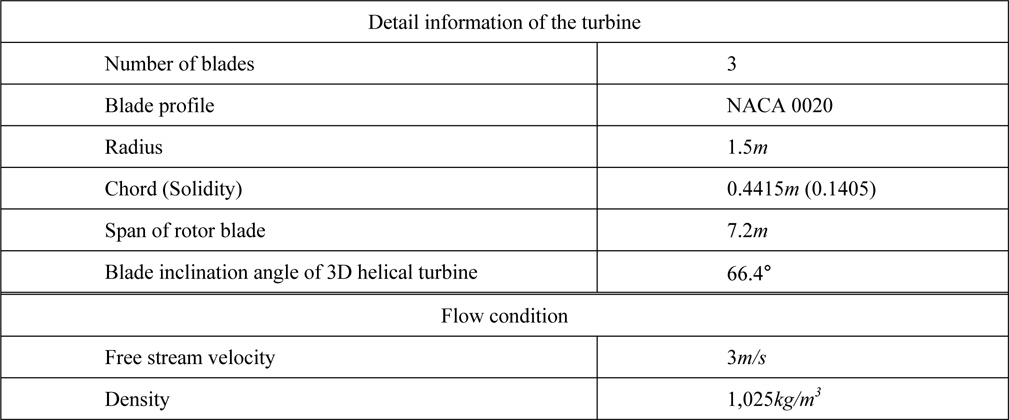
Two-dimensional (2D) computational fluid dynamics (CFD) simulations are frequently used for designing sections of a Darrieus vertical-axis turbine (VAT). Previous work involving 2D CFD simulations (KORDI, 2011) conducted a parametric study of the hydrofoil profile, the number of blades, the solidity, and the diameter. Through this parametric study, an optimal design with three blades was obtained with respect to the power coefficient, fluctuation, and other parameters. The detailed information pertaining to the turbine model is summarized in Table 1. The diameter of the turbine was 3m, the sections used were the NACA 0020 with a chord length of 0.4415m, and the solidity was 0.1405. A free stream velocity of 3m/s is chosen because most tidal turbines are designed with a range of 2m/s to 4m/s; this type of turbine was developed for installation into the Uldolmok narrow channel of Korea, which is known to have high flow speeds. The operating speed of the turbine is normally expressed as the tip speed ratio (TSR), which is defined as ωR /V , where ω is the angular velocity, R is the radius of the turbine, and V is the incoming velocity. A sliding mesh is utilized for modeling the rotation of the turbine. In order to use the sliding mesh method, the computation domain is divided into two domains: (1) the outside domain with the inlet velocity, outlet pressure, and symmetry boundary conditions on side surfaces; and (2) the inside domain near the blades with the wall boundary. Between two domains, an interface condition is applied. The domain sizes for 2D and 3D models are shown in Fig. 1. A structural mesh with a viscous length of the mesh expressed as y⁺ < 5 is recommended around the wall of the blade when the k-ω SST turbulent model accounts for the wall function by default. A zoomed view of the mesh near the wall is also included in Fig. 1.

The power coefficient of the turbine is estimated through two simulation methods in this study. First, a CFD simulation with the TSR given, similar to methods in other numerical studies, was used. Here, the rotational speed of the turbine axis is specified by user input. Second, a CFD simulation with a given load, that is called a flow-driven rotor simulation, is used. It is similar to an experimental approach, in which the rotational speed of the turbine axis is not fixed, but the turbine is rotated at a certain velocity upon the hydrodynamic moment on the blade, the inertia moment of the blade, and the given counter moment on the rotational axis. The instantaneous power generated by the turbine is equal to the product of the angular velocity (ω) of the turbine and the torque (T ) acting on it. The power is not constant because the torque and velocity are not constant in the Darrieus VAT. Hence, the average power per cycle is calculated as the product of the average values of these terms per cycle, as shown below

The power coefficient ( C_p ) is then defined as

where A is the frontal area of a turbine, which is equal to the product of the turbine diameter and height in a 3D model or only the turbine diameter in a 2D model; V_∞ is the free stream velocity; and ρ is the fluid density at far field boundary condition.

Another quantitative value used to express the performance of a Darrieus VAT is the torque ripple factor (TRF), which is defined as the ratio of the peak-to-peak amplitude of the instantaneous torque to the torque averaged in one cycle, as follows:

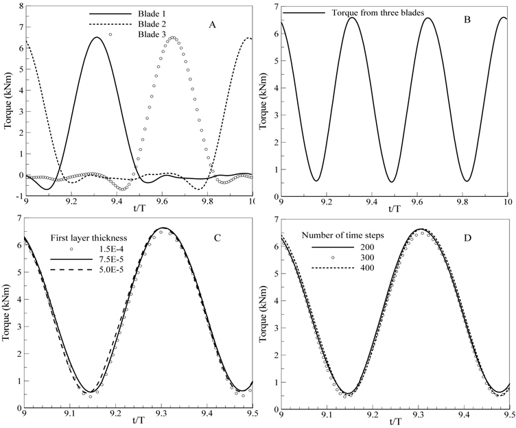
The numerical result is sensitive to the mesh quality in the boundary layer; hence, additional studies are necessary to check for numerical convergence before conducting further simulations. The dependence of the numerical result on the grid size and time step in a simulation with a TSR of 2.5 is shown in Fig. 2. The torque variation of each blade and the summation of three blades per cycle are respectively shown in Figs. 2(A) and Figs. 2(B), while the dependence of the torque on the mesh size and the number of time steps during a half cycle are presented in Figs. 2(C) and Figs. 2(C)(D), respectively. The degrees of mesh independence are studied with using three levels: coarse (69720 nodes), medium (129450 nodes) and fine (229371 nodes), corresponding to the first layer thickness from the wall, of which the values here are 1.5E-4m, 7.5E-5m and 5E-5m, with the viscous lengths, y⁺, set to 5. Similarly, the independence of the number of time steps on the numerical solutions is investigated by three levels: 200 steps, 300 steps and 400 steps per cycle. The differences between them are ignored. According to the results, 200 time steps and a medium-level mesh (129450 nodes) are chosen for the following 2D simulations.

In contrast to a simulation with the TSR given, the rotational speed of the blade (ω) is not specified in an unsteady flowdriven rotor simulation. In a flow-driven rotor simulation, the turbine blade rotates around its axis at a certain rotational speed by balancing the hydrodynamic moment, the moment of inertia, and the imposed counter moment on the turbine. When the angular position of the turbine blade is notated by θ , the angular velocity and the acceleration of the turbine are θ′ and θ′′. The rotational motion of the turbine around its axis is determined by the following equation

where J is moment of inertia of the turbine, M_F is the total hydrodynamic moment acting on the turbine blade and M_A is the applied moment on the rotational axis for determining the power of the turbine. Hence, the rotational speed of the blade (ω) is defined as follows:

In the numerical set-up, a six-degree-of-freedom (6DOF) solver (ANSYS, 2010) is utilized through a user-defined function (UDF) to analyze the rigid-body dynamics. The 6DOF solver calculates the hydrodynamic moment by integrating pressure and shear stress on the surface of the turbine blade in other to estimate the motion of a rigid object. Hence, we have to specify the moment of inertia of the turbine blade as well as the constraint of the turbine’s motion in the x, y, and z directions in the UDF.

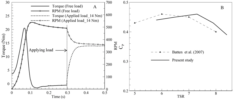
First, to benchmark the flow-driven rotor simulation, the experimental data of a HAT with an 80cm diameter in a cavitation tunnel (Batten et al., 2007) are used. These are known as some of the best data measured from experiments with a three-blade HAT. A free stream velocity of 1.73m/s, a tunnel domain, the NACA 63-8xx series turbine blade profile with a pitch angle of 20° are used in the experiment as the input conditions in a three-dimensional simulation. Fig. 3 shows as well the curves of the torque and the rotational speed of the turbine, which we could predict from an experimental study. The rotational speed of the turbine quickly accelerates from 0 to a high RPM and then gradually decreases in a free load condition. Afterwards, it is significantly reduced to a lower RPM when counter torque is imposed on the turbine axis. A RPM curve with very low fluctuation after the reduction, which is known as one of the main advantages of a HAT, is obtained by a numerical simulation. These characteristics of the RPM curve are different in a VAT, as shown in the next simulation in this study. When comparing the results of the flow-driven rotor simulation with the experimental results, the values of C_p are shown to be close to each other, as shown in Fig. 3, although the positions of the peak C_p differ slightly in the two cases. The maximum of the power coefficient, 48%, is achieved when the TSR ranges from 6 to 7.

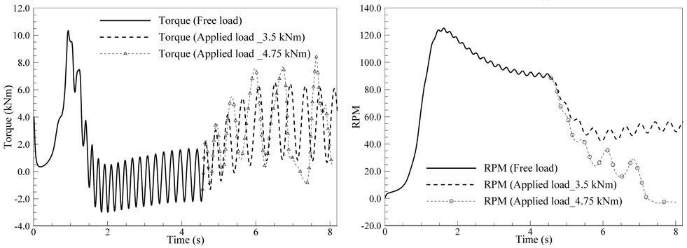
First, a 2D flow-driven rotor simulation of the Darrieus turbine is conducted to ascertain its performances quickly and compare them to those of a simulation with a given TSR. The simulation conditions are summarized in Table 1. The mass and moment of inertia of the turbine which made of aluminum, are utilized in the UDF. The torques and RPMs of the Darrieus turbine are shown in Fig. 4. Briefly, the figure presents the performance of the turbine under three different load conditions: a free load condition and two applied load conditions with counter torques T of 3.5kN⋅m and T of 4.75kN⋅m per unit length. The free load condition initially is a case in which no counter torque is applied to the turbine axis and where the turbine accelerates to around 125 RPM under hydrodynamic moment from the flow and then decelerates to about 90 RPM, from t = 0.0s to 4.56s. Low self-starting capability due to the need to overcome the inertia of a large turbine is well known as one of the main disadvantages of a straight-bladed turbine (Shiono et al., 2002), which is also demonstrated by slow acceleration in the beginning of the RPM curve. From the initial state, the turbine accelerates slowly from t = 0.0 to 0.6s and the rotational speed then increases from 0 RPM to 15 RPM. Afterwards, it accelerates rapidly, with the rotational speed finally reaching a maximum value of 125 RPM at t = 1.5s. Subsequently, the rotational speed gradually reduces to a convergent value, 90 RPM, with low fluctuation. When counter torque of 3.5kN⋅m is applied to the turbine axis at t = 4.56s, the rotational speed decreases significantly and then gradually increases to a new convergent value of 52 RPM. By multiplying the counter torque and the rotational speed, the corresponding power coefficient is 0.48. As shown in the torque curve, high fluctuation of the torque on the axis of the turbine is observed. This is also another main drawback of a Darrieus VAT. If a high counter torque such as 4.75kN⋅m is applied, the rotational speed of the turbine is dramatically reduced and the turbine starts to rotate in the opposite direction in what is known as an over-loading condition. This is shown in the lower subfigure in Fig. 4.

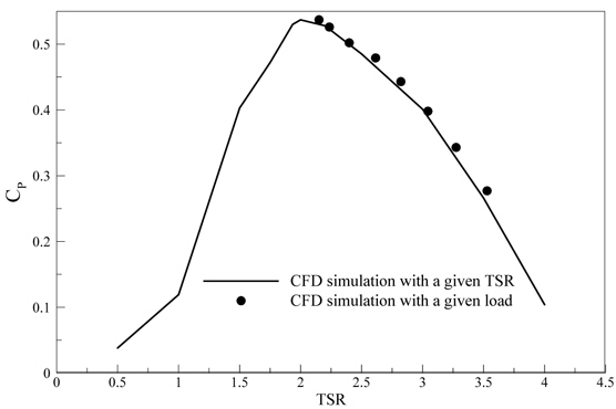
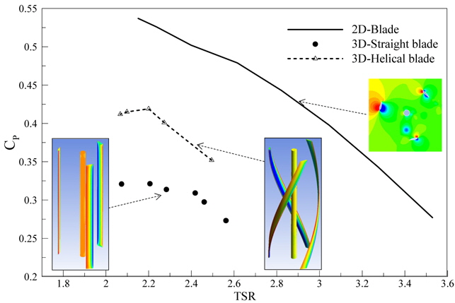
The power coefficient of the Darrieus turbine predicted by the 2D flow-driven rotor simulation is depicted when counter torque is imposed with different values, as shown in Fig. 5. For a comparison, the power coefficient predicted from a simulation with the TSR given is also plotted. The results from both simulations are in good agreement; the maximum power coefficient is nearly 0.535 when the TSR is around 2. There is a small gap between the TSRs when using these two approaches. The power coefficient cannot be predicted when the TSR is less than 2 in the flow-driven rotor simulation, which is considered as an overloading condition, for example, with counter torque of 4750N⋅m, as shown in Fig. 4. It is speculated that the over-loading condition arrives at a somewhat small value of the imposed torque due to the 2D assumption.

Here, the performance of the Darrieus turbine is investigated through two configurations with the same height: a straightbladed and a helical-bladed turbine. Additional information is also shown in Table 1. The height of the turbine is 7.2m and the height-to-diameter ratio of both turbines is 2.4. The inclination angle of the helical-bladed turbine is defined as

where n, h, and d are number of blades, the span of the rotor blade and the diameter of the rotor (Shiono et al., 2002), respectively. Our helical-bladed turbine has an inclination angle of 66.4°; hence, its blades cover 360° from a top view. The ratio and inclination angle were sourced from a previous study (KORDI, 2011). The domain of the 3D simulation is shown in Fig. 1, and 1,512,783 nodes are used after the grid convergence is checked. As in the 2D simulation, the 3D flow-driven rotor simulation requires the moment of inertia of the aluminum turbine for the six-DOF solver, which is connected via UDF to the flow solver. Fig. 6 shows a comparison of the power coefficients of both turbines along with the 2D turbine. The maximum power coefficients of the helical-bladed and straight-bladed are were respectively 0.42 and 0.33 at a TSR of approximately 2.2, which are 22% and 38% lower than that of the 2D turbine, respectively. These results indicate that 3D tip effect is significant and that the helical blades enable the turbine to extract more power from the tidal flow due to the inclination angle. Previous studies also showed that the power coefficients from the 3D simulation and the experiment were nearly half of those from a 2D CFD estimation (Mohamed, 2012; Raciti et al., 2011).

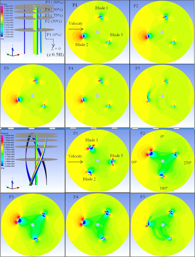
Fig. 7 presents the pressure distribution in the cross-sections of planes 1, 2, 3, 4, and 5 from the middle to the tip positions along the vertical axis corresponding to z/0.5H values of 0%, 50%, 75%, 90%, and 99%. The 3D tip effect is clearly shown in the straight-bladed turbine according to the decrease in the pressure difference near the blades when the cross-section moves toward the blade's tip. More specifically, it can be seen that the difference in the positive and negative pressure levels shows a slight reduction from planes 1 to 2, after which they sharply decrease from planes 2 to 4. Moreover, the difference of the pressure levels is nearly nonexistent on plane 5. The pressure distribution on plane 1 is similar to that in the 2D CFD simulation; therefore, the difference between these planes can explain a major gap in the power coefficients between the 2D and 3D models shown in Fig. 6.

For the helical-bladed turbine, the azimuth blade angle along the vertical axis is different in each section. Thus, the characteristics of the pressure contours are clearly different from those in the straight-bladed turbine. The 3D tip effect is only apparent between the pressure contours in planes 4 and 5, while the other planes show different characteristics due to their different azimuth angles. In detail, from planes 1 to 3, the NACA section of blade 1 moves from 0° toward 90° in terms of the azimuth blade angle; therefore, the difference in the negative and positive pressure zones near blade 1 becomes greater. The pressure contours near blades 2 and 3 also depend on their azimuth blade angles. Regarding the straight-bladed turbine, the position of the NACA section was identical in all planes; therefore, the pressure contours in all sections show similar pressure differences. In addition, the pressure contours in the circular area inside the three blades present different characteristics of the flow in the helical-bladed and straight-bladed turbines; the green color shown is dominant in the case of the helical-bladed turbine; thus, its pressure is lower than that of the straight-bladed turbine. Subsequently, the helical-bladed turbine could absorb more energy from the tidal flow than the straight-bladed turbine due to the large difference between the inside and outside pressure levels.

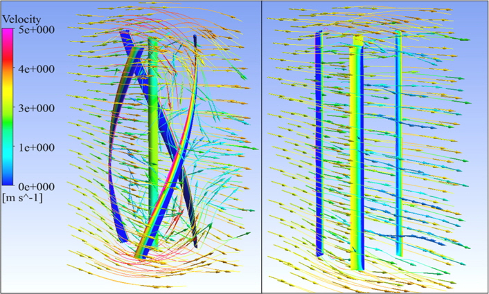
Fig. 8 shows the flow velocity vectors over the two turbines, demonstrating how the helical geometry affects the streamlines. The flow has strong mutual interaction with the three blades before it moves downstream. Thus, the streamlines are strongly deformed in terms of their direction when they pass through the helical-bladed turbine, whereas only small deflections are observed in the case of the straight-bladed turbine. The differences in the streamlines between the two 3D turbines mainly cause the differences in the pressure distribution of each section and in their power coefficients.

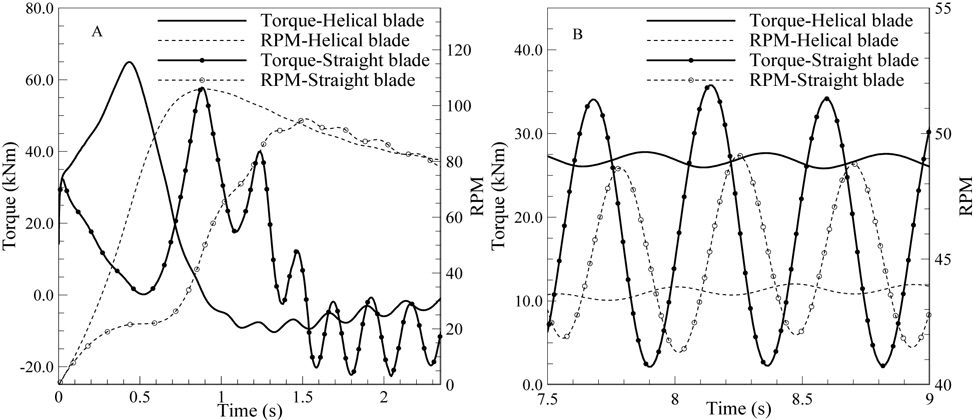
The helical-bladed turbine is known to have advantages over the straight-bladed turbine in terms of its self-starting capability and the reduced fluctuation of its torque curve, as visually exhibited by the 3D flow-driven rotor simulation shown in Fig. 9. Fig. 9(A) shows the hydrodynamic torque on the rotational axis of the turbines with the RPM in the free load condition. In the beginning, both of the turbines were forced to rotate under high hydrodynamic torque, 32kN⋅m, with the RPM increasing from 0. Next, the torque continues to increase from 32kN⋅m to 65kN⋅m until t = 0.45sec, and the RPM increases sharply to its maximum value of 105 at t = 0.9sec in the helical-bladed turbine. In contrast, the torque is reduced from 32kN⋅m to 0kN⋅m until t = 0.5sec in the straight-bladed turbine. Meanwhile, the RPM increases from 0 to 20 until t = 0.3sec, becoming nearly constant between 0.3sec and 0.6sec in the straight-bladed turbine. Afterwards, the torque on the straight blades increases rapidly from 0kN⋅m to 57kN⋅m between 0.5sec and 0.9sec, and the RPM reaches its maximum value of 95 at t = 1.5sec. After reaching the maximum value, both the RPM and the torque decrease to their convergent values in both turbines. Due to the high fluctuation of the torque, the acceleration in the early stage of the straight-bladed turbine is delayed compared to that of the helical-bladed turbine; thus, the helical-bladed turbine shows greater self-starting capability than the straight-bladed turbine. In other words, the self-starting capability is improved by the helical blade because the duration required to reach the maximum rotation speed for the helical-bladed turbine is shorter (0.9sec) than that of the straight-bladed turbine (1.5sec).

Fig. 9(A) shows the hydrodynamic torque on the rotational axis of the turbines and the RPM when the maximum power coefficients of the helical-bladed and straight-bladed turbines are 0.42 and 0.33, respectively. The average TSR was approximately 2.2 when the corresponding counter torque levels are 26.8kN⋅m and 20kN⋅m on the helical-bladed and straight-bladed turbines, respectively. Clearly, the torque curves present another advantage of the helical-bladed turbine over the straight-bladed turbine in the form of the low fluctuation of the torque. In detail, the torque ripple factors (TRF) are 0.065 and 1.675 in the helical-bladed and straight-bladed turbines, respectively. The RPM curves also show high fluctuation in the straight-bladed turbine. Using similar definitions of TRF, the RPM ripple factors are 0.0057 and 0.077 in the helical-bladed and straight-bladed turbines, respectively. In sum, the torque and RPM curves of the helical-bladed turbine are much smoother than those of the straight-bladed turbine.

As noted above, the main advantage of the Darrieus VAT is its ability to generate power from the flow in any direction without any yawing control as compared horizontal-axis turbine which is mainly used in tidal steam generators (Beri and Yao, 2011). A straight-bladed Darrieus VAT is advantageous given its simple manufacturing process and assembly stages. However, researchers should consider how to overcome the two main drawbacks of the straight-bladed Darrieus turbine: its low self-starting capability and the high fluctuation of the torque on its turbine axis. There are several experimental and numerical approaches that seek to overcome these drawbacks. These include a cambered foil to enhance the self-starting capability and an increase in the number of blades to reduce the fluctuation of the torque (Castelli et al., 2012; Hwang et al., 2009). Thus far, the utilization of helical blades is one of the most promising solutions to accomplish these goals. Recently, throughout in-situ experiments, a helical-bladed turbine has been proven to offer continuous high performance in South Korea (Han et al., 2013). Our work is among the first to present a quantitative assessment of the performance of the helical-bladed Darrieus turbine using a flow-driven rotor simulation, which provides operational characteristics close to those of an actual experiment as compared to a simulation with a given TSR. The advantages of the helical-bladed turbine are demonstrated through a direct comparison with the straight-bladed turbine of the same size. First, the helical-bladed turbine shows an improvement in the self-starting capability with higher torque levels and with less time required to reach the maximum RPM as compared to a straight-bladed turbine. Next, the fluctuation of the torque acting on the rotational axis during the power extraction stage is significantly reduced; that is, the TRF is reduced from 1.675 to 0.065 while the RPM remains nearly constant. The power coefficient also is improved from 33% to 42% in the given conditions of the Darrieus turbine. Consequently, an improvement of the self-starting capability and a reduction of the fluctuation by the helical-bladed turbine are clearly demonstrated as compared to a straight-bladed turbine in flow-driven rotor simulations. The improvement of the power coefficient by the helical-bladed turbine may be dependent on the operating conditions or on blade characteristics such as the pitch control, which is known to improve the power coefficient of Darrieus turbines (Hwang et al., 2009; Schönborn and Chantzidakis, 2007). An improvement of the power coefficient of Darrieus turbines is the subject of our future study.

In this study, flow-driven rotor simulations are conducted in an effort to investigate the operational characteristics of a Darrieus turbine which can be captured in an actual experiment instead of a simulation with a given tip speed ratio (TSR). Specifically, the self-starting capability, fluctuation of the torque and the RPM characteristics while also considering an over-loading condition are clearly demonstrated in a flow-driven rotor simulation. Two-dimensional (2D) computational fluid dynamics (CFD) simulations initially show that the power coefficient predicted from a flow-driven rotor simulation is in very good agreement with the prediction from a simulation with a given TSR. Next, the three-dimensional (3D) effect on the power coefficient of Darrieus turbines is explored in detail by comparing the results from 2D and 3D simulations. Finally, through 3D CFD simulations for an optimal design, the helical-bladed turbine shows prominent advantages over a straight-bladed turbine of the same size, including an improvement in its self-starting capability and the minimization of the fluctuation of the torque levels and RPM while extracting power as well as an increase of its power coefficient from 33% to 42% under the given operating conditions. Eventually, in the design stage of a Darrieus turbine, it is certain that a flow-driven rotor simulation can provide more information than a simulation with a given TSR before expensive experimental work.