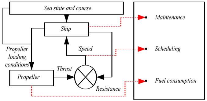
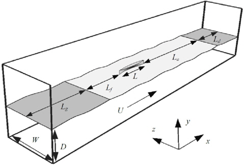
The performance of a ship when travelling in a seaway has always been a hot topic. This is true now more than ever with ever increasing requirements for environmental performance and rapid transit of goods. The introduction of the Energy Efficiency Design Index (EEDI) as a design constraint for new ships from 2013 (IMO, 2011) is likely to lead to an increased need for design modifications that lead to improved efficiency without negatively impacting other factors such as transport capacity, safety, etc. Accurately predicting performance in waves and being able to judge the impact of subtle design changes is therefore identified as an area of high interest. From a hydrodynamical point of view, understanding the interaction between the ship, the sea state that it is in and the propeller that is powering it will give an answer to most questions regarding performance. A schematic of this interaction created by Windén (2012) is shown in Fig. 1.
To properly model this interaction, strong linking is needed between flow conditions around the hull and the performance of the propeller. Currently, the only method that allows for detailed flow features around the hull and the propeller to be modelled is a Navier-Stokes (NS) based solver.
One reason why proper verification and validation of NS based modelling of ships in waves is hard to achieve is the complexity of the model itself. For self-propulsion, a way to model the rotating propeller has to be added on top of the already complex dynamical geometry. This leads to a difficulty in identifying the most important sources of error. For example incorrect phasing of forces and motions has been identified as a problem in recent workshops (Larsson et al., 2014). If the motions are seen to be out of phase, it is hard to tell if this is due to incorrect forcing, a problem with the mesh deformation scheme or the coupling scheme between forces and motions. This means that the predicted propulsive performance of the ship has many associated error sources and it may be hard to clearly quantify the underlying reason for the error.
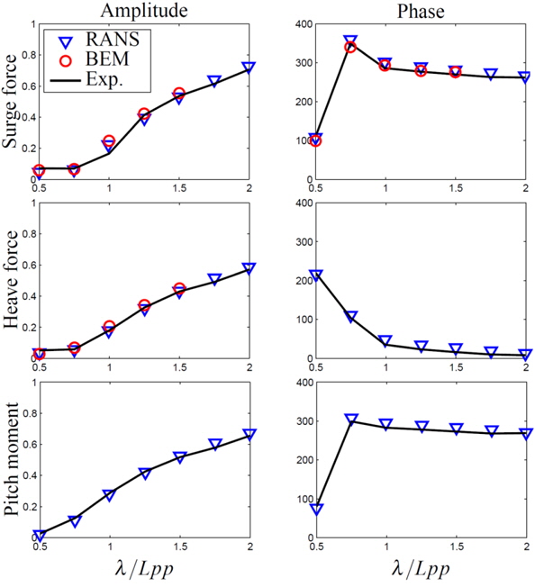
One of the most well adopted ways to address a problem with many unknowns is to start with something that is known or can be found out easily and gradually build understanding from this. Applying this reasoning to the problem of modelling ship performance in waves means removing many of the uncertainties mentioned above. RANS is chosen as a modelling technique due to its advantage in computational efficiency over other NS based methods. A validation study based on experiments by Journée (1992) of the forces and moments on a fixed Wigley hull in waves predicted using the open source CFD software OpenFOAM has been carried out by Windén et al. (2012). Fig. 2 shows encouraging results for the prediction of the amplitude of the forces at different wavelengths but a problem with the phasing still remains even when the hull is fixed. The study also compares results with a nonlinear Boundary Element Method (BEM) by Kjellberg (2011) which seemed to predict the phasing slightly better while giving a greater error in predicting the amplitudes of the forces.
The next step after the forces and moments are validated is either to study the motions or to study propulsion. In this paper, the second issue is addressed. The objective is to identify more about what factors should be considered when modelling selfpropelled ships in waves using RANS. In the simulations in this paper, the model is free to surge and the RPM of the propeller is controlled using a PID-controller. This means that the influence of the propeller thrust on the surge for different control conditions can be studied.
The setup of the numerical towing tank is shown in Fig. 3. The size of the computational domain is set so that
The mesh is created using an automated refinement strategy described by Windén et al. (2012). The final mesh size lies around 6M cells with a
• an adequate distribution of cells in the free surface region • adequate refinement around the hull, in the wake and in the propeller region • smooth blending between the refinement in these two areas where they intersect
The particulars of the chosen hull are shown in Table 1.
[Table 1] Particulars of tested hulls.

Particulars of tested hulls.
where a2 gives the shape of the hull as

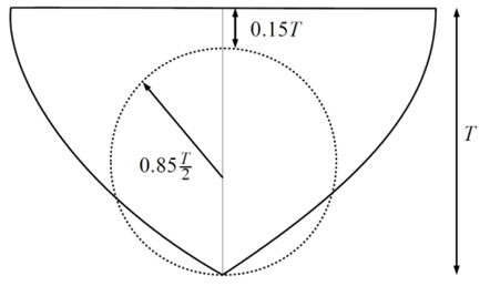
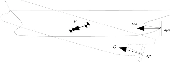
The Wigley hull is a purely academical hullform and has no consideration of propeller positioning in the definition of its shape. The propeller disc is therefore positioned half a radius behind the aft perpendicular, with a lower point flush with the keel and with a diameter of 85% of the draught. This is seen as representative of a typical positioning of the propeller on a ship. The positioning of the propeller disc relative to the rear profile of the used Wigley hull is shown in Fig. 4. Furthermore a hub with a radius of 10% of the total disk radius is used as well as a shaft extending into the hull and ending in an ellipsoid cap to minimise separation.
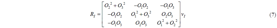
The propeller is modelled using a body force approach, meaning that an external force is added to the RANS momentum equation to represent the work done on the fluid by the propeller. The body force due to the propeller

In Eq. (2), the left hand side represents the momentum change of the fluid. The average velocity components are denoted as
The magnitude and direction of

and the planar shift of the centre of gravity due to motions is denoted

and the orientation of the propeller axis

A cell is given a non-zero value of

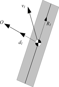
The local radius of cell
The definitions of
From this definition it follows that

>
Thrust and torque distribution
The body force exerted on a certain cell within the propeller disk can be calculated in several ways. The most accurate representation is to model the lift and drag of the blades along radius by separating them into finite elements, each having a certain foil shape and attitude to the oncoming flow. This is known as Blade Element Momentum theory (BEMt.) Simplifications to this can be made by allowing the blades to sweep over a certain distance to give average values in larger sectors of the disk. A further step is to assume that the propeller rotates fast enough for the thrust and torque to be smeared over the entire disk at any given time step. The approach to modelling the blades depends on the amount of information is needed about the instantaneous effect of the blades on the surrounding fluid. This must be put in relation to the time scales of other phenomena around the propeller such as vortices separating from the stern area and how well the interaction of these with the propeller is to be modelled.
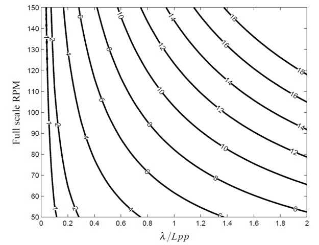
In this case the frequency of the waves passing and thus the variations in resistance and surge are deemed most important. The relation between the passing period of wave crests e T at different
As seen in Fig. 7, there will be more than 4 rotations of the propeller for every wave encounter in most situations. For low values of

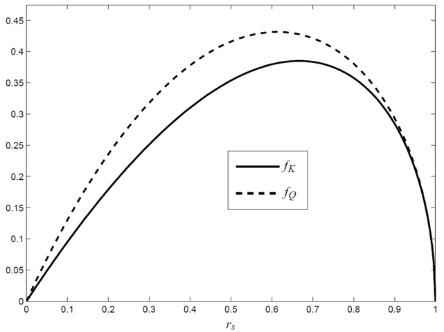
A shape function describing the thrust distribution is given as

and equally for the torque

The shape functions
The shape functions are normalized so that the summation value over the entire disk corresponds to the desired thrust and torque


where

The direction of rotation can be altered by replacing Eq. (14) with

The body force for a cell

The thrust and torque are decided by the coefficients of thrust and torque


Since the propeller blades are not explicitly modelled in this case, the variation of


In this case, the inflow speed is taken as the base forward speed

In Eq. (21), care must be taken with the signs of
Eqs. (17) and (18) as well as the shape functions (Eqs. (10) and (11)) assume that the flow into the propeller is uniform so that the local advance ratio is constant along the circumference. If the propeller is working behind a hull, the wake created by the ship will distort this condition. The thrust and torque varies periodically because of the surging motion through Eq. (21). However, the presence of the waves would also mean a periodic variation of thrust and torque due to an unsteady wake, something that is not considered here. By applying a BEMt method post run-time to estimate the thrust and torque variations behind the Wigley hull in this study, Windén et al. (2013) found a thrust variation of 16% around the mean value due to the unsteady wake.
Since the thrust produced by the propeller is a function of the RPM, it is possible vary the RPM based on given criteria for the thrust. In the interest of maintaining a constant service speed in waves, the RPM can be varied as to maintain the thrust needed to keep constant forward speed. Since the undisturbed forward speed is modelled with a current in this case, keeping constant speed is equivalent with keeping zero surge motion.
This can be achieved in two ways. The most direct approach is to iterate in each time step to find the thrust that will ensure force balance in the surge direction. The other alternative is to use a control function to steer the RPM towards the correct value based on information available from previous time steps. The second approach is preferable here, both in terms of computational time but, more importantly because it more closely represents a situation that could be applied on a real ship. Because of the nonlinear properties of marine propulsion systems, to achieve optimal propulsion performance it is necessary to apply some sort of control algorithm to govern the propeller RPM (Xiros, 2002). This is particularly important when ship dynamics are also considered as a factor (Kashima and Takata, 2002). A similar approach as the one described in this paper with a body force propeller and PID regulator for the RPM was applied by (Carrica et al., 2008) for studying broaching events.
The PID controller is defined by letting the RPM in a time step be a function of the RPM in the previous time step and a correction value based on an error

An appropriate definition of the error
To accentuate the connection with the resistance, the acceleration is multiplied by the mass of the ship to give an estimate of the current force acting on the hull. Furthermore, to avoid motion with constant velocity (in this case meaning that the hull moves with constant velocity other than the one specified) a penalty of 1000 is put on the integral value of acceleration. The error is now defined as

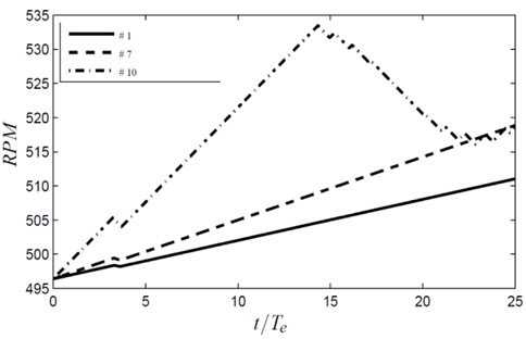
In addition to the PID-controller governing the RPM, some restrictions must be applied to make the simulation more realistic. The RPM should not be allowed to exceed a certain value since that would mean a great risk of cavitation and damage to machinery in a real propulsion system. Furthermore, large acceleration of the propeller rotation should also be disallowed since the torque needed to achieve such acceleration lies beyond the capability of both engines and propeller shafts. Furthermore, RPM increases are usually limited in marine engines to avoid large heat gradients etc. A typical maximum value for how fast the propeller rotation is allowed to change is around 1 RPM per minute in full scale. If the example scale factor of 40 is applied in this case, this is equivalent to a maximum increase of 0.67 RPM/s in model scale. Furthermore, typical working shaft-RPM for most large merchant vessels lie between 40 and 100 RPM. This corresponds to between 250 and 630 RPM in the example model scale.
Simulations are started from an initialised solution where the steady wave pattern of the hull is allowed to develop. At the initial state, the resistance is recorded and the starting RPM is set as to match this resistance with a corresponding thrust. The hull is then subjected to regular waves with the first crest reaching the hull about
[Table 2] PID coefficients and initial RPM value.

PID coefficients and initial RPM value.
All the information about the propeller extent and position are shown in Table 3
[Table 3] Positioning and extent of propeller.
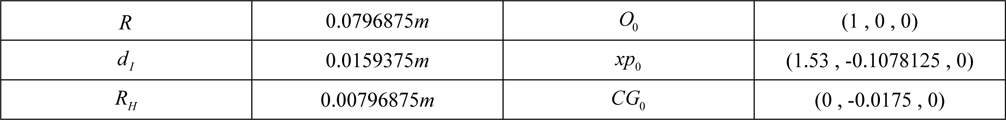
Positioning and extent of propeller.
Nine different values on the maximum permissible RPM change rate
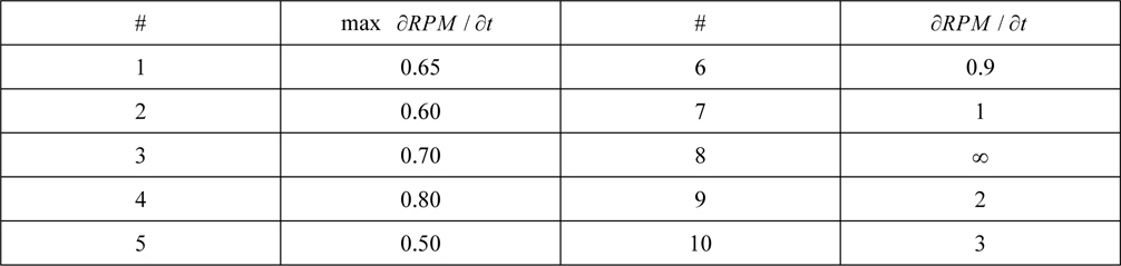
RPM constraints.
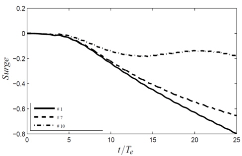
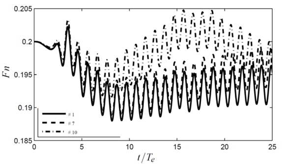
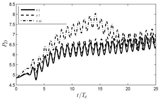
Controllers 2-5 performs similarly in terms of surge motion compared to controller 1, significant differences are only found for controllers 6-10. In Figs. 9, 10 and 11, the forward speed, surge and RPM for controllers 1, 7 and 10 are shown. Finally, the delivered power, which can be calculated as
As seen in Fig. 9, the hull experiences a periodical oscillation in forward speed due to the waves. There is also a drop in the mean velocity. This is due to the mean increase in resistance due to waves
As seen in Figure 10, even though the hull returns to its initial forward speed, the integral value of the velocity means that it has been given a large distortion in surge. While this is not a problem in real applications, in this case it means that the mesh has been distorted. In the interest of accuracy future implementations should take this into consideration.
If the actual powering performance in waves is sought, it would not be suitable to construct a controller that puts a penalty on the surge drift. Instead it would be preferable to initialize the simulation from a fixed hull in waves and use the RPM needed to overcome
The controller function described in this paper is a simplified version which mostly serves to demonstrate the opportunities of using open source RANS modelling with external inputs to more closely represent real operating conditions. Much more advanced controlling algorithms could be employed here, see for example Xiros (2002). Furthermore, the actuator disk model has many limitations. To properly include the propeller geometry and to draw more detailed conclusions about the effects of unsteady loading, a BEMt approach is preferred. The future aim for this model is to replace the actuator disk formulation with the BEMt model developed by Phillips et al. (2009; 2010).
This study has shown that it is possible to model and discuss around several aspects of self-propulsion using the described method. There is however need for proper validation against experimental data to ensure the accuracy of the model. The benefit of using RANS CFD to do this rather than experimental methods is that the entire flow field can be accessed and analysed to study the influence of e.g. changes in bow and stern shape and the subsequent change in performance. The future goal is to apply the methodology described in this paper to more realistic hull forms to be able to conduct detailed studies on more of the factors affecting ship performance in waves.
Finally, the conclusions drawn regarding the controller constraints may become relevant with future engine development (with for example fuel cell powered electrical engines) where the RPM increase should be able to happen faster than with current marine diesels.