Motion planning has been an essential part of robotics for a long time. Many algorithms have been developed, which develop a plan for a robot to move from the initial configuration to the target configuration. Nevertheless, algorithm complexity has been a challenge for real-life applications.
The development of motion planning from graph search algorithms [1] and has led to the modern complicated sampling-based algorithms [2]. Dijkstra’s algorithm is one of the simplest and basic algorithms for finding paths on a graph. One of the approaches for the construction of a motion plan in a configuration space is to discretize the space with hyper-cubes and then, execute a graph search algorithm on a discrete structure. However, in practical applications, this approach can rarely be used for tasks with high dimensionality, because the algorithm complexity increases exponentially.
An extension of Dijkstra’s algorithm, which is called A* [1], introduced heuristics for graph-search algorithms to significantly improve the algorithm’s performance in terms of the computation time, depending on the task.
The other successful approach for motion planning in a high-dimensional space is the Rapidly Exploring Random Tree algorithm [3]. This algorithm rapidly extends a tree structure in a high-dimensional space and has proved to be efficient in many practical applications. However, it suffers in the presence of narrow paths. Various methods have been proposed to overcome this problem [4].
However, in recent years, more attention has been drawn to the area of experience-based planning, because tasks have become increasingly complicated. Re-planning strategies in similar environments are covered in [5-7]. Trajectory libraries approaches are covered in [8-10].
Heuristics are applied in many practical motion planning tasks. However, as planning problems become increasingly difficult, the complexity of heuristics increases, and designing a heuristic itself becomes a challenging task.
The main contribution of this work is the development of an approach for the algorithmic generation of heuristics. The work is done in the following steps: • Represent a motion planning algorithm’s interaction with the environment as a random process. • Represent a heuristic as a distribution of random variables that control the random process of planning. • Since a heuristic is usually developed by humans on the basis of their knowledge about the type of environment or the type of task. Assume that knowledge about environment is the knowledge of the distribution of obstacles in the environment. • Apply machine learning to learn the distribution of obstacles in typical environments. Utilize the learnt distributions as a heuristic to control the extension of a motion planning algorithm.
In the experimental section, the designed heuristic is applied to different types of motion planning algorithms in order to show the performance improvement.
II. PROPOSED METHOD DESCRIPTION
>
A. Heuristic and Distribution of Obstacles
Let us consider an example of motion planning in a two-dimensional space for a point mass in a free space. The shortest path would be a straight line, connecting the initial and the target configurations. The shortest path is different from a straight line, if there are obstacles between the initial and the target points. Therefore, obstacles do affect the final plan.
Now, let us analyze an example of planning in a real environment with obstacles. Let us have an intelligent agent
To illustrate the above idea, let us consider an example of a robot, which navigates on the ground. Let us model the surrounding physical world as a set of tuples {
We can also model the above-mentioned world with random variables
Basic planning algorithms without heuristics are designed to be systematic and sufficiently universal to deal with any kind of input problems. Thus, they consider that obstacles are distributed uniformly. However, in fact, if obstacles have some pattern and are not distributed uniformly, then the planner may work inefficiently. This has led to the introduction of various heuristics to make planning algorithms solve particular problems more efficiently.
Let us represent the interaction between a planner and an environment as a random process. As a heuristic controls the behavior of this interaction at every cycle of the algorithm, the heuristic is considered to be a distribution of the possible actions that the planner could perform.
It should be noted that a heuristic may be deterministic with respect to some calculated values, and have conditional entropy equal to zero (e.g., the A* algorithm), but due to the randomness of obstacles, the full entropy of the heuristic may be more than zero.
The main idea behind this work is as follows: If a human designs a heuristic for a particular task, then it means that he/she tries to model a probability distribution function of the actions that the planner would take. In the proposed approach, we try to model this probability distribution function algorithmically, with the help of machine learning.
>
B. Generalized Planning Framework
To further analyze motion planning algorithms and heuristics, let us describe a generalized planning framework.
It is an algorithm template that may be instantiated to describe most of the modern sampling-based planning algorithms. See Algorithm 1.
This function generates a pair {
The generalized framework may be extended to be a random tree, with configurations sampled according to some random distributions. Algorithm 2 is an extension of a template for a randomly built tree. Nodes
This graph extension strategy is itself sufficiently general, because it can model other sampling-based planning algorithms in terms of the distributions of random variables
EXAMPLE 1:
The generalized algorithm may also be utilized to implement the well-known Rapidly Exploring Random Trees (RRT) [4]. The extension of the function
EXAMPLE 2: RRT may be modeled by biasing distributions of
We can conclude from these two examples that biasing of the distribution of
For the study presented in the given work, we apply machine learning algorithms to find the distribution of the variable
III. EXPERIMENTS AND DISCUSSION
This section describes how heuristics may adapt to the given typical environment by learning. Learning is implemented as finding the probability distribution function of a planner’s parameters from the observations of a typical environment.
In previous sections, sampling-based planners were generalized to a tree structure, which expands in a search space. The expansion is parameterized in two ways. The first is which a node is selected to be extended, and the second is the selection of the control input to be applied to the extending node.
In the presented experiment, the second parameter is utilized to improve the performance of a planning algorithm. The control input is learned from the observations of successfully generated paths. RRT was used to generate the paths for the observations.
After the probability distribution function was approximated with the sum of the Gauss distributions with learned means, it was applied to the sampling of the control input.
In order to show that z planner with applied self-learning heuristics performs better, we applied the proposed strategy to different sampling-based planners. Planners were selected to differ in the way nodes for extensions are selected. In the first case, we utilized the uniform random selection of nodes from the whole tree. In the second case, we utilized the selection of nodes for rapid expansion in space. The probability that a node is selected is proportional to the volume of the Voronoi cell that corresponds to the node.
All the algorithms were run 10 times. The number of iterations, number of failed collision checks, and path lengths were recorded. In the first run, the algorithms were run until the path was found. In the second run, planning was run for a fixed number of iterations.
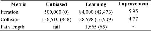
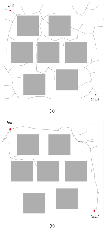
The results of the experiments with random node selections are shown in Tables 1 and 2. As is apparent, random node selection is inefficient, and an unbiased algorithm could not find the solution even after 500,000 iterations. Self-learning heuristics improved the performance of the planner, and thus, it could find a solution. The boundaries of exploration can be seen in Fig. 1.
[Table 1.] Performance of self-learning heuristics applied to random tree search algorithm

Performance of self-learning heuristics applied to random tree search algorithm
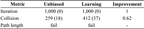
Performance of random tree search algorithm with self-learning heuristics when the number of iteration is fixed
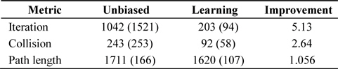
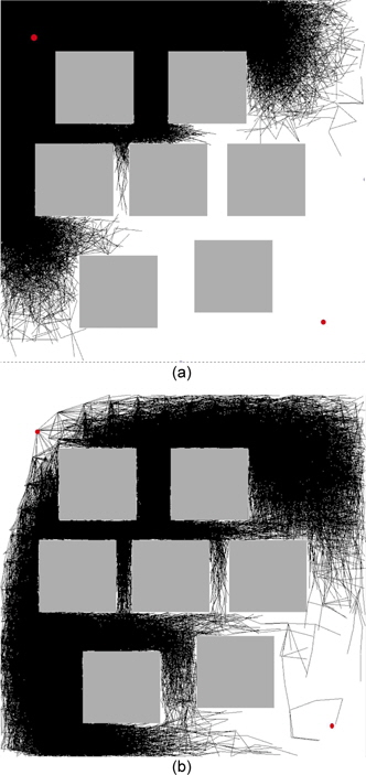
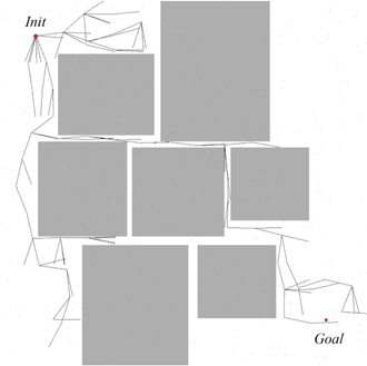
The results of the experiments with rapidly expanding node selection are shown in Tables 3 and 4. This strategy extends the algorithm faster. An unbiased version of the algorithm is in fact an implementation of an RRT algorithm. Self-learning heuristics improved the performance of the planner, and thus, it could find the solution faster as shown in Fig. 2. Planning is performed from the initial point in the left top corner to the goal point in the right bottom corner.

Performance of self-learning heuristics applied to the search algorithm with Voronoi cell volume-based node selection
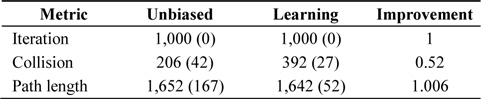
Performance of the search algorithm with Voronoi cell volume-based node selection and self-learning heuristics when the number of iteration is fixed
Unlike expected, the self-learning heuristics caused more collision check fails during the test with a fixed number of iterations (See Table 2). In both cases, motion planners failed to reach the goal; therefore, the number of iterations was considerably small. If compared to the results from Table 1, it may be seen that the self-learning heuristic experiences relatively few collision failures before it reaches the target.
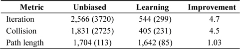
The same experiments were also performed on a similar map, with a considerably narrower distance between squares; see Fig. 3. The result is presented in Table 5. As expected, the original RRT’s performance started to drop significantly. In our experiments it sometimes took more than 10,000 iterations and the algorithm still could not find the solution. Because of these failures, the average number of iterations is high. In all three experiments, the algorithms enhanced with self-learning heuristics improved the performance of the original algorithm.

Results of running algorithm, until a path is found, on a map with narrow paths: random tree with Voronoi cell volume-based node selection: comparison with and without self-learning heuristics
In this work, we have proposed a method, which allows heuristics for a motion planner to be generated by a computer by observing the results of prior successful planning tasks in the environment. We have experimentally shown that if planning algorithms are generalized and parameterized with two random variables, then the observation of the distribution of these parameters on successful paths may be utilized to create a heuristic. The proposed method was applied to different sampling-based planning algorithms in different environments, and in all cases, it showed performance improvements.