The past few years have witnessed the emergence of applications that monitor streams of data items, such as sensor readings, network measurements, stock exchanges, online auctions, and telecommunication call logs [1-4]. In these applications, fast, approximated results are more meaningful than delayed, accurate results. For example, consider a medical center where biosensors are used to monitor the body status of patients. In this example, a life-threatening event should be detected on time, and notified to the medical staff immediately, even if it proves to be a false alarm. Delayed detection of critical events is unacceptable. Similar examples can be found in network intrusion detection, plant monitoring, and so on.

Stream monitoring applications do not fit the traditional database model. Data streams are potentially unbounded. Therefore, it is not feasible to store an entire stream in a local database. Also, queries posed to a database system may not be answered, because an input stream can be infinite. Instead, stream applications adopt the notion of continuous queries. In this scheme, queries over data streams run continuously over a period of time and incrementally return new results, as new data arrives.

For example, consider a query that asks for the maximum value of sensor readings over the latest 30 seconds. This can be specified as a structured query language (SQL)-like query Q1, where window specification is defined in square brackets.

Q1. SELECT MAX(value) FROM Sensors [RANGE 30 seconds]

During run time, the query is evaluated for each tuple arrival. Whenever a new tuple arrives at time t, windowing tuples is first performed: tuples whose timestamps are within (t – 30, t] belong to the current window, and other tuples are discarded. Then, the maximum sensing value over tuples in the window is calculated. The same process is repeated, whenever a tuple arrives on the input stream.

As shown in the example, continuous queries generally use sliding windows , to limit the scope of query processing to recent data [3-6]. From this, the queries can be answered over unbounded data streams, even when they involve blocking operators, such as joins and aggregates—operators that cannot start processing until entire inputs are ready.

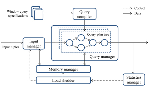
Fig. 1 shows a system structure to process window queries. The query processing engine is also called a data stream management system (DSMS). Well-known examples of the system include Aurora [1], STREAM [4], TelegraphCQ [7], Gigascope [8], NiagaraCQ [9], and StreamMill [10]. The system can be viewed as a real-time processing engine with the support of an SQL interface, which enables users to specify their applications in a declarative fashion. It consists of the following components:

● Query compiler translates user-specified window queries into a query plan tree. The plan tree can be viewed as a filter, through which input streams pass. As mentioned above, queries specified for stream applications can be characterized as window queries (Section Ⅱ).● Query manager runs the generated plan trees over input data streams. Some parts of the trees can be shared to reduce execution time (Section Ⅲ-A). The behavior of stateful operators, such as aggregates and joins, can differ from those in the traditional DBMSs (Section Ⅲ-B). The operators in the plan trees can be scheduled dynamically, according to changing system status (Section Ⅲ-C).● Memory manager provides storage for input tuples and intermediate results generated from the operators in plan trees. It is organized to maximize the sharing of tuples, to avoid disk accesses by reducing memory size (Section Ⅲ-A).● Load shedder monitors system status including arrival rates of input tuples and memory growth during query execution. If the system is overloaded, it prompts the memory manager or the input manager to discard some portion of the tuples (Section Ⅲ-D).● Input manager synchronizes multiple data streams (for a join) and resolves disorder of the streams. Disorder control is necessary to clearly determine the boundaries of sliding windows and to avoid tuple discards that can occur from windowing tuples (Section Ⅲ-E).

In this paper, we provide an overview of data stream processing. In what follows, we consider the specifications and processing of stream queries. We also review related work in this area.

So far, many query languages have been proposed to specify stream queries, including AQuery [11], the box and arrow scheme [1] in Aurora, CQL [5] in STREAM, StreaQuel [7] in TelegraphCQ, and ESL [10] in Stream- Mill. There are also the special-purpose query languages that are used in Gigascope [8] and Tribeca [12].

In Aurora [1], users construct query plans via a graphical interface by arranging boxes corresponding to query operators, such as selections, joins, and aggregates. The boxes are connected with directed arcs to specify data flows. The boxes can be rearranged in the optimization phase. On the other hand, most other systems including STREAM support SQL-like languages for query specification. The query languages have syntax to specify sliding windows to deal with unbounded data streams. This section focuses on the specification of window queries.

A real-time data stream is a sequence of data items that arrive in some order (e.g., timestamp order). In the STREAM project [2, 4, 5], assuming a discrete time domain T, a stream is defined as follows.

DEFINITION 1 (Stream). A stream S is a possibly infinite bag (multiset) of elements (s, t), where s is a tuple belonging to the schema of S, and t ∈ T is the timestamp of the element.

A relation is also defined with the notion of time, which is different from the conventional relation.

DEFINITION 2 (Relation). A relation R is a mapping from T to a finite bag of tuples belonging to the schema of R.

To denote a relation at any time instant t ∈ T, R(t) is used. In the window query model, an unbounded stream is translated into finite relations using windows. Suppose that the latest tuple arrives at a certain time τ for query Q1. Then, R(τ) will consist of tuples whose arrival timestamps are in the interval of (τ − 30, τ]. The aggregate max will then be applied to R(τ). In this example, R(·) will be updated, whenever a new tuple arrives.

The relation R(·) can be organized differently, if a different type of window is applied to the query. The window models can be classified according to the following criteria [3, 7].

● Movement of the window's endpoints: Two fixed endpoints define a fixed window, while two sliding endpoints define a sliding window. One fixed endpoint and one moving endpoint define a landmark window.● Physical vs. logical: Physical or time-based windows are defined in terms of a time interval, while logical or count-based windows are defined in terms of the number of tuples. The latter windows are also called tuple-based windows.● Update interval: Eager re-evaluation updates the window whenever a new tuple arrives on a stream, while lazy re-evaluation induces a jumping window. If the update interval is larger than or equal to the window size, the window is called a tumbling window.

If sliding windows are used in a query, the query becomes monotonic. Let A(Q, t) be the answer set of a window query Q at time t, and 0 be the starting time. The query is then re-evaluated over newly arriving tuples, and qualifying tuples are appended to the result. The answer set of Q at time t can be represented as follows.

On the other hand, if landmark windows are used, the query will be non-monotonic. It will be recomputed from scratch during every query re-evaluation. The answer set of Q at time t can be represented as follows.

To specify a sliding window, the syntax proposed in [6] can be used. In the syntax, a window can be defined with three parameters: 1) RANGE, to denote a window size; 2) SLIDE, to denote a slide interval of the window; and 3) WATTR, to denote a windowing attribute—the attribute over which RANGE and SLIDE are specified.

In general, time-based sliding windows are most commonly used in stream applications [13, 14]. The previous query Q1 is an example of a time-based window with a size of 30 seconds. A tuple-based window can also be defined with the RANGE parameter. The following shows a query to compute the max value over the latest 100 tuples.

Q2. SELECT MAX(value) FROM Sensors [RANGE 100 rows]

To define an update interval for the window, the SLIDE parameter can be used. The following query updates the max value every 30 seconds, which is calculated over tuples arriving for the latest 30 seconds. The query is an example of the tumbling window.

Q3. SELECT MAX(value) FROM Sensors [RANGE 30 seconds, SLIDE 30 seconds]

Note that, with time-based windows, the window interval is determined based on the arrival timestamp of the last input tuple. On the other hand, windowing can also be performed based on different attribute values, not only arrival timestamps. For instance, a user may want to perform the windowing based on the tuples' generation timestamps. Let the attribute denoting a tuple's generation timestamp be sourceTS. To use it for windowing, a WATTR parameter can be used as follows.

Q4. SELECT MAX(value) FROM Sensors [RANGE 30 seconds, SLIDE 30 seconds WATTR sourceTS]

The following query shows another example of using the WATTR parameter. The query will be posed to identify the list of product names of the latest 10 orders issued from customers.

Q5. SELECT productName FROM Orders [RANGE 10 rows, WATTR orderId]

When a windowing attribute is explicitly specified, as in Q4 and Q5, input tuples may not be in an increasing order of the windowing attribute. This is because input tuples may experience different network transmission delays. Out-of-order input tuples complicate the identification of window boundaries and contents. To simplify this job, existing approaches usually discard out-of-order tuples. These tuple drops may lead to inaccuracy in aggregate queries. This issue will be discussed in Section Ⅲ-E.

To chain a number of relevant queries, the concept of named queries was introduced in STREAM. Consider that we want to identify congested segments on a highway. The highway is divided into a number of segments with exit and entrance ramps at each segment boundary. In this example, each vehicle periodically transmits its speed and position measurements. Suppose the schema of the measurements is PosSpeedStr(vid, speed, pos), where PosSpeedStr is the name of the input stream. The attributes vid, speed, and pos denote the id of a vehicle, its speed in miles per hour (MPH), and its position on the highway in feet, respectively.

To calculate the number of vehicles in each segment, the position of a vehicle should first be converted to its corresponding segment number. Assume that segments are exactly 1 mile long. Then, the segment number can be computed by dividing pos by 1760. The query for this purpose can be specified as Q6, named SegSpeedStr. The name of a query usually comes ahead of the SELECTFROM-WHERE clause.

Q6. SegSpeedStr SELECT vid, speed, pos/1760 as segno FROM PosSpeedStr

From SegSpeedStr, the congested segments can be identified. Suppose that a segment is considered congested, if the average speed of vehicles in the segment in the latest 5 minutes is less than 40 MPH. Then, a query to identify congested segments can be constructed as shown in Q7. For the complete description of this Linear Road Benchmark example, refer to Arasu et al. [5] and Jain et al. [15].

Q7. CongestedSegRel SELECT segno FROM SegSpeedStr [RANGE 5 minutes] GROUP BY segno HAVING AVG(speed) < 40

As shown in this example, the outputs of a query Q_i can be fed to other queries Q_j, by specifying the name of Q_i in the FROM clause of Q_j. Using this scheme, complex application requirements can be specified by chaining a number of simple named queries without introducing a nested query.

This section discusses the issues in processing of window queries over continuous data streams. The discussion consists of query plan structure, blocking operators, operator scheduling, load shedding, and disorder control.

A user-specified window query is translated into a plan tree from the query compiler (Fig. 1). The structure of a query plan is similar to one in a traditional DBMS. In general, a query plan consists of three types of components:

● Query operators: Each operator reads a stream of tuples from one or more input queues, processes the tuples based on its semantics, and writes the results to a single output queue.● Inter-operator queues: A queue connects two different operators and defines the path along which tuples flow, as they are being processed.● Synopses: An operator may have one or more synopses to maintain states associated with operators. For example, a join operator can have one hash table for each input stream as a synopsis.

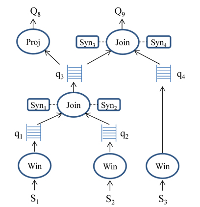
Fig. 2 illustrates plans for two queries, Q8 and Q9. The plans consist of six operators denoted by ovals, four synopses syn₁ to syn₄, and four queues q₁ to q₄. Query Q8 is a projection over a join of two streams S₁ and S₂. Query Q9 is a join of three streams S₁, S₂, and S₃. For all input streams, the same sliding windows are given, which are 30 seconds long. Then, the two query plans can share a subplan joining windowed streams of S₁ and S₂.

Q8. SELECT id, value FROM S1 [RANGE 30 seconds], S2 [RANGE 30 seconds] WHERE S1.id = S2.id

Q9. SELECT * FROM S1 [RANGE 30 seconds], S2 [RANGE 30 seconds], S3 [RANGE 30 seconds] WHERE S1.id = S2.id and S2.id = S3.id

S2 [RANGE 30 seconds], S3 [RANGE 30 seconds] WHERE S1.id = S2.id and S2.id = S3.id

Synopses are maintained for stateful operators, such as joins or aggregates. Simple filter operators, such as selections and duplicate-preserving projections, do not require a synopsis, because they need not maintain state. For synopses, various summarization techniques can be used, including reservoir samples [16], sketches [17], wavelets [18, 19], and histograms [20].

Queues are generally organized to have pointers to tuples stored in the memory manager (Fig. 1). An operator reads the pointers from its input queues and accesses tuples through the pointers. If a queue is shared by multiple operators (e.g., q₃ in Fig. 2), tuples in the queue can be discarded only when they have been read by all parent operators. From this, the size of a shared queue depends on the rate at which the slowest parent operator consumes the tuples. If consumption rates of parent operators are significantly different, it is preferable not to share a subplan [4].

As mentioned earlier, query operators can be stateless or stateful. The behavior of stateless operators is the same as in a traditional DBMS. On the other hand, the behavior of stateful operators can differ. When stateful operators are involved in stream queries, sliding windows are needed to decompose infinite streams into finite subsets and produce outputs over the subsets. In this section, we focus on aggregates and joins with sliding windows.

To compute window aggregates, many existing algorithms use the divide-and-conquer approach. For example, a dataset X is divided into disjoint subsets X₁, X₂, ..., X_n, where . Then, an aggregate over X, f(X), is computed using sub-aggregates over X_i, as shown in the following equation. Below, g(·) and h(·) are some aggregate functions.

f(x) = h(｛g(X_i)┤|1≤i≤n｝)

For any possible sub-aggregate function g(·), if there is no constant bound on the size of storage needed to store the result of g(·), the function f(·) is holistic. The examples of holistic aggregates include MEDIAN, QUANTILE, and MODE. Otherwise, the function can again be classified into distributive and algebraic [21]. If g(·) and h(·) are equal to f(·), the function is distributive. Examples include SUM, COUNT, MAX, and MIN. Otherwise, the function is algebraic. AVG is algebraic, since it can be computed using SUM and COUNT.

Li et al. [22] proposed an approach for evaluating aggregate queries when sliding windows are overlapping. When adjacent windows overlap, a stream is divided into disjoint subsets called panes. The panes are also called basic windows in the literature. The size of a pane can be obtained by GCD(V_R, V_S), where V_R is the value of a RANGE parameter, and V_S is the value of a SLIDE parameter in a window specification. Window-level aggregates can then be computed from pane-level sub-aggregates. For example, consider a query to find the maximum bid price for the past 4 minutes and update the result every minute. This query can be described as follows.

Q10. SELECT MAX(bid-price) FROM Bids [RANGE 4 minutes, SLIDE 1 minute]

Given Q10, a pane becomes a 1-minute-length subwindow (Fig. 3). The method computes the max bid price for each pane. The max price for each window can then be obtained from the max values of four panes that contribute to the window. This approach can be applied to the other aggregate functions mentioned above.

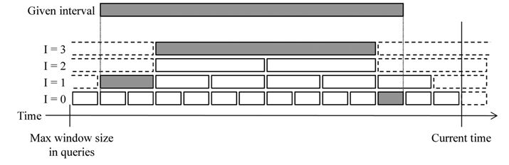
Arasu and Widom [23] proposed resource sharing techniques, when a number of window queries are posed over the same data. In their method, a time interval is divided into a number of predefined smaller intervals called base intervals. The base intervals form a basis for intervals: any interval can be expressed as a disjoint union of a small number of base intervals (Fig. 4). Using this property, any f(I) can be computed using a small number of precomputed f(I_b) values, where I is a window interval in a query, and I_b is a base interval.

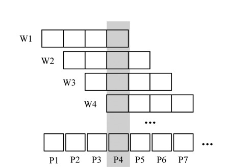
When discussing join algorithms, sliding window equijoins are most commonly considered [24, 25]. Suppose we want to join m input data streams over a common attribute A. Let the i-th input stream be S_i (1 ≤ i ≤ m), and its window size be W_i (i.e., the value of a RANGE parameter). At time t, a tuple s belongs to a windowed substream Si[Wi], if s has arrived on S_i in time interval (t − W_i, t]. An m-way window equijoin can then be represented as S₁[W₁] ⋈_A S2[W2] ⋈_A ... ⋈_A S_m[W_m]. The output of the join consists of all m pairs of tuples, (s₁, s₂, ..., s_m), satisfying s₁.A = s₂.A = ... = s_m.A, where s_i ∈ S_iW_i]. The windowed substream S_i[W_i] is also called a javascript:;window extent.

Consider Q8, which is a join of two streams S₁ and S₂. In this case, windows slide with each tuple arrival because only RANGE parameters are given in the window specifications. Subsequently, the join is evaluated whenever a new tuple arrives in any input stream. Its algorithm can be described as follows.

Algorithm 1. Sliding window equijoinWhenever a new tuple s arrives on Sk (1 ≤ k ≤ m), 1. Update all Si[Wi] (1 ≤ i ≤ m) by discarding expired tuples 2. Join s with all Si[Wi] (i ≠ k) 3. Add s to Sk[Wk]

The algorithm consists of three steps: windowing streams (step 1), producing join results over window extents (step 2), and adding the new tuple to its window extent (step 3). Assuming a symmetric hash join, step 2 can be described in more detail:

2.1. Hash: calculate a hash value v for s2.2. Probe: scan all hash tables of Si (i ≠ k), to see if matching tuples with value v exist in the tables2.3. Output: generate results, if matching tuples exist in all hash tables

Previous work [24-26] showed that a symmetric hash join is faster than any tree of binary join operators, emphasizing that its symmetric structure can reduce the need for query plan reorganization. From this, an m-way symmetric hash join is commonly considered in data stream processing.

There has been substantial research in joining data streams. Early studies in this area focused on a binary join. Kang et al. [27] showed that when one stream is faster than the other, an asymmetric combination of hash join and nested loop join can outperform both the symmetric hash join, and the symmetric nested loop join. Golab and Ozsu [24] showed that hash joins are faster than nested loop joins, when performing equijoins. Assuming that the query response can be delayed up to a certain time, they discussed eager and lazy evaluation techniques for a window join.

The discussion was extended to a multi-way hash join, in a study by Viglas et al. [25]. They proposed MJoin, a multi-way symmetric hash join operator and showed that the m-way hash join is faster than any tree of binary join operators. That idea was developed into AMJoin, proposed by Kwon et al. [28, 29]. AMJoin improves the performance of MJoin, by detecting join failures in advance. In AMJoin, unnecessary probes for hash tables can be avoided by using a bit-vector hash table, where each table entry has a bit-vector, denoting whether matching tuples exist in all streams.

The window join was also used to track the motion of moving objects, or detect the propagation of hazardous materials in a sensor network. This idea was captured by Hammad et al. [30]. The same authors also proposed scheduling methods for query operators, when a window join is shared by more than two branches of operators in a query plan tree [31]. Hong et al. [32] discussed techniques for processing a large number of extensible markup language (XML) stream queries involving joins over multiple XML streams. The method focused on the sharing of representations of inputs to multiple joins, and the sharing of join computation.

Query plans are executed via a global scheduler, which runs each operator in query plans, to help move tuples through the plans and produce results. The simplest scheduling scheme is the round-robin, where operators run in a circular order, and each operator runs until it consumes all tuples in its input queue. This method is easy to implement, and starvation-free, but far from optimal.

In many stream management systems, more intelligent scheduling techniques have been proposed and used, including train scheduling [1] in Aurora, eddies [33, 34] in TelegraphCQ, and chain scheduling [35] in STREAM. The first two methods focused on improving throughputs, while the objective of the last was to minimize peak memory size (i.e., peak total queue size).

In Aurora, the contents of inter-operator queues can be written to disk, which is different from STREAM. Therefore, to improve performance of query execution, context- switching between operators should be minimized. For this purpose, their scheduling algorithm (called train scheduling) focused on 1) generating long trains of tuples, 2) processing complete trains at once, and 3) passing them to subsequent operators, without having to go to disk. By batching the processing of tuples through operators, they attempted to reduce I/O overhead.

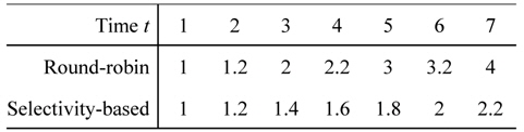
In TelegraphCQ, query scheduling is conducted by eddies [33]. An eddy is a highly adaptive query processing operator that continuously re-optimizes a query, in response to changing runtime conditions. It does this by treating query processing as the routing of tuples through operators and making per-tuple routing decisions. The cost of making per-tuple routing decisions might be high, which has been asserted by various parties. Regarding this, Deshpande [34] implemented eddies in a Postgre- SQL open source database system in the context of a TelegraphCQ project and showed that the overhead of the eddy mechanism was negligible.

The chain scheduling in STREAM focused on minimizing a peak total queue size during query processing. For this purpose, they considered the selectivity of each operator in query plan trees. Consider the following simple example. Suppose we have a query plan with two unary operators, O₁ and O₂: O₁ receives tuples from input queue q₁ and writes its output to q₂, which connects to the input of O₂. Let the selectivity of O₁ be 20%, i.e., it consumes n tuples from q1 in one time unit, and introduces n/5 tuples into q₂. Also assume that O₂ takes one time unit to operate on n/5 tuples. Then, there are two possible scheduling strategies:

● Round-robin scheduling: Tuples are processed to completion in the order they arrive at q1. Each batch of n tuples in q1 is processed by O1 and then O2, requiring two time units overall.● Selectivity-based scheduling: If there are n tuples in q1, then O1 operates on them using one time unit, producing n/5 new tuples in q2. Otherwise, if there are any tuples in q2, then up to n/5 of these tuples are operated on by O2, requiring one time unit.

Suppose we have the following arrival pattern: n tuples arrive at every time instant from t = 1 to t = 7, then no tuples arrive from t = 8 to t = 14. On average, n/2 tuples arrive per unit of time, but with an initial burst. Fig. 5 shows the total size of queues q₁ and q₂ under the two scheduling strategies during the burst, where each entry is a multiplier for n. As shown in this example, selectivity- based scheduling is clearly preferable in terms of runtime memory overhead during the burst. Babcock et al. [35] extended this scheme to the chains of operators within a query plan (i.e., the groups of operators in query paths), when making scheduling decisions.

Due to the high arrival rate of tuples, memory may not be enough to run queries. In this case, some portion of input or intermediate tuples can be moved out to a disk or can simply be discarded from memory to shed system load. In data stream management systems, the latter approach is generally adopted, because in many stream applications, fast, approximate results are considered more meaningful than delayed, exact answers.

The load shedder in Fig. 1 continuously monitors memory status. If memory is inadequate, it determines 1) in which query plan operators load shedding occurs and 2) how many tuples should be discarded at that point in the plan. Tatbul et al. [36] discussed the problem of determining these two points. In most cases, tuple drops occur at the entry of query plan trees (e.g., input manager) to maximize the effect of load shedding. In their work, the number of tuples to be discarded is estimated based on quality-of-service (QoS) specifications (e.g., importance of tuple values). Babcock et al. [37] discussed the same problem for aggregate queries. Their method focused on minimizing the degree of inaccuracy introduced in query answers. Al-Kateb and Lee [38] considered load shedding for temporal queries and proposed a new accuracy metric for their load shedding decision.

There has also been substantial research in operatorlevel load shedding. Many studies focused on load shedding in join operators. When memory is not enough for the join, victims should be chosen from the synopses of a join operator (e.g., hash tables). According to victim selection strategies, load shedding algorithms for window joins can be classified into the following three models.

● Frequency-based model [26, 39-42]: The priority of a tuple s is determined in proportion to the number of tuples in windows, whose value is the same as that of s.● Age-based model [43]: The priority of a tuple is determined based on the time since its arrival, rather than its join attribute values.● Pattern-based model [29]: The priority of a tuple is determined based on its arrival pattern in data streams (e.g., the order of streams in which the tuple appears).

Das et al. [26] proposed the concept of semantic load shedding, as opposed to random load shedding. In semantic load shedding, join attribute values are considered to maximize a user-defined similarity measure. They considered the MAX-subset measure, which maximizes the number of tuples in the approximate output of the join. The MAX-subset measure was considered for load shedding in many algorithms [40-42]. Das et al. [26] also proposed two heuristics to determine the priority of tuples in an online join: PROB and LIFE. The former discards the tuple with the lowest probability to join with a partner tuple in the other stream. The latter discards the tuple with the lowest product of its remaining lifetime and the probability that it joins with another tuple.

On the other hand, Srivastava and Widom [43] showed that the frequency-based model (e.g., PROB) is not appropriate in many applications and proposed an agebased model for them. In their model, the expected join multiplicity of a tuple depends on the time since arrival, rather than its join-attribute value. Their method focused on the memory-limited situation. Many other studies including [26, 40-42] also assumed the memory-limited situation, and then discussed their load shedding algorithms. On the other hand, Gedik et al. [39, 44] emphasized a situation where the CPU becomes a bottleneck (i.e., when an input arrival rate exceeds CPU processing speed), and then proposed load shedding techniques to shed the CPU load.

Kwon et al. [29] considered the load shedding problem for applications where join attribute values are unique, and each join attribute value occurs at most once in each data stream. For these applications, the frequency-based model cannot be used. To resolve this issue, they proposed a new load shedding model, in which the priority of a tuple is determined based on its arrival pattern in data streams (e.g., the order of streams in which the tuple appears).

A data stream is an ordered sequence of data items. The order is important in windowing data streams. In general, window operators assume that tuples arrive in an increasing order of their WATTR values. Out-of-order tuple arrivals are ignored to facilitate the identification of window boundaries [1, 6]. However, tuples may not arrive in the WATTR order, since they often experience different network transmission delays. These out-of-order tuples are discarded in the windowing phase, and such tuple drops can lead to inaccurate results in aggregate queries.

To resolve this issue, input tuples are buffered in the input manager (Fig. 1), until they can be outputted without violating violating the WATTR order. To determine which tuples can go out, the notion of punctuations [45] can be used. A punctuation p is an assertion indicating that no more tuples with attribute value p will be seen in the future.

Heartbeats [13, 46] can be viewed as special kinds of punctuation, where attributes are timestamps of tuples. Heartbeats can be estimated internally in the system or can be given externally from remote stream sources, such as routers. Ding et al. [47] and Li et al. [6] assumed that heartbeats were externally given, and proposed methods for processing join or aggregate queries gracefully. However, external stream sources may not provide heartbeats in real-world applications. In addition, the heartbeats themselves can be out-of-ordered, when stream sources are in remote locations.

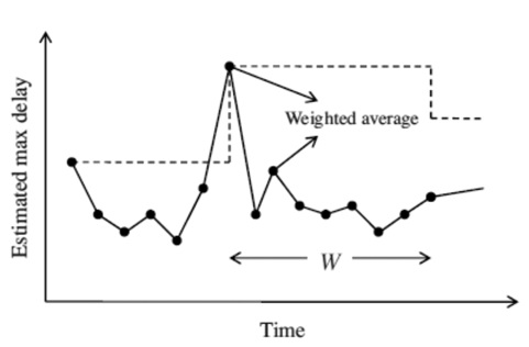
When estimating heartbeats internally, existing approaches generally use the maximum network delay seen in the streams. Let the max delay until time t be m. Then, the heartbeat is estimated to t – m, and all tuples with generation timestamps smaller than t – m are outputted from the buffer. The k-ordering mechanism [48], the skew bound estimation [14], the timestamp mechanism in Gigascope [8, 13], and the ordering mechanism in NiagaraCQ [9] are similar to this approach.

The heartbeat estimation algorithms focus on saving as many discarded tuples as possible. Consequently, they tend to keep the buffer size larger than necessary. For example, the adaptive method proposed by Srivastava and Widom [14] estimates the max delay m by(m₁ + m₂)/2, where is the max delay seen in the stream at time t, and m₂ is the second max delay seen for the W interval of time from t (Fig. 6). We can easily see that m is kept large most of the time, since it is determined by the two largest values of network delays seen in the stream in a certain period of time.

To resolve this issue, Kim et al. [46] proposed a method to estimate the buffer size based on stream distribution parameters monitored during query execution, such as tuples' interarrival times and their network delays. In particular, their method supports an optional window parameter DRATIO (an abbreviation for a drop ratio), to enable a user to control disorder according to application requirements.

Q11. SELECT MAX(value) FROM Sensors [RANGE 30 seconds, DRATIO 1%]

The query above specifies that the percentage of tuple discards permissible during query execution should be less than or equal to 1%. By specifying DRATIO, a user can control the quality of query results according to application requirements; a small value for the drop ratio provides more accurate query results at the expense of high latency (due to a large buffer), whereas a large value gives faster results with less accuracy (from a smaller buffer).

In this survey, we have tried to coherently present the major technical concepts for data stream processing. To keep the task manageable, we restricted the scope of this paper to the specification and processing of window queries. This is meaningful, because most major stream processing engines, such as Borealis [49] (the successor of Aurora), STREAM, TelegraphCQ, and StreamMill, support an SQL interface, to receive application requirements in the form of window queries [50]. The discussions in this paper included synopses structures, plan sharing, blocking operators, operator scheduling, load shedding, and disorder control.

Many interesting issues related to data stream processing could not be included in this survey, for example:

● Classification and clustering● Frequent pattern mining● Synopsis structures, such as reservoir samples, sketches, wavelets, and histograms● Indexing streams● Multi-dimensional analysis of data streams

Some of the issues were discussed in other papers. For example, Gaber et al. [51] presented a survey related to mining data streams. Aggarwal and Yu [52] provided a survey on synopsis construction in data streams. Mahdiraji [53] provided a survey on the algorithms for clustering data streams. These surveys can augment the discussions given in this paper.