Schema matching plays an important role in the realm of data integration, which is a solution for sharing multiple heterogeneous data sources through a unified access interface. In essence, the schema matching problem refers to the problem of finding semantic correspondences, also called matches, between elements of the source schema, and elements of the target schema. A match means that its two elements hold the same meaning, or refer to the same object. The match is very significant for creating a unified mediated schema over multiple source schemas, exchanging data from one schema to another schema, and sharing data in a similar domain. The schemas to be matched are typically designed by different developers, who have different habits and experiences, so the schemas often have diverse structures and representations, and this makes schema matching difficult. In addition, dozens of tables and thousands of attributes in the schemas also increase the difficulty of schema matching. Even with the availability of some domain expertise, the task of schema matching may not be easy.
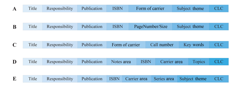
Much attention has been paid to schema matching, and a multitude of techniques, also called matchers, have been proposed, e.g., [1-5]. However, these existing matchers are not infallible, because no matcher is perfect and returns matches with 100% accuracy. Consequently, additional efforts are required for schema matching. In this paper, we proposed a novel matching technique that exploits the order of attributes appearing in the schema structure of query results, to discover the matches between the attributes of the source schema, and the attributes of the target schema. As is well known, the words in almost every book we can read in English, are arranged from left to right, and this is a habit of people, to capture information from left to right. For example, given a spreadsheet listing records about books, people will always start from the first column to read, then the second column, etc. The departure times in the grid of train schedules are typically arranged at a position closer to the left side with respect to arrival times. The field ‘name’ will be arranged at the left side of the field ‘nationality’ in the database table ‘student’. Examples like this are numerous. In a sense, the reading habit can be viewed as a preference of readers. As a result, the developers of applications for structured information always design the schema structure according to this habit. That is, the more important columns will be arranged in positions closer to the left side. For example, the column ‘bookname’ in the above spreadsheet may appear on the left-hand side of the column ‘author’; as such, the column ‘student name’ will be arranged on the left side of the column ‘gender’ in the student table. It is reasonable that the important information is the first received by readers. The arrangement of these columns not only embodies the reading habit, but also the default rule of some industries. We browse five digital libraries, and pose the same query to their respective databases, then present the schema structures of their returned results about books in Fig. 1. Surprisingly, all these libraries arrange the attributes of the book in almost the same order. It is easy to see that the attributes close to the left side are arranged according to reading habit. However, the extent of importance among the attributes close to the right side is almost the same, but they also have a similar order. The reason for this behavior is that these libraries fall into the same industry, where there exist some default rules. Consequently, we are able to exploit these habits, which are typically conformed to by both schemas to be matched, to find matches.
As is clear from the discussion above, different attributes have different importance in structuring the query results to be shown to the final users. As a result, an attribute with different importance will hold its own position in the schema structure of the query results. Actually, the appearance order of attributes refers to the positions of attributes appearing in the schema structure. It is normal that the positions of an attribute in some query results are likely to differ slightly, because of lack of generality. However, positions of an attribute in numerous query results will reflect the reading habit (designing method of developers), which we talk about. Thus, the statistics about the appearance order of an attribute in a large number of query results can be seen as its identification, differing from other attributes. Every query result corresponds to one query statement in the query log. Consequently, to collect statistics about attributes, we will start with the query logs. The core idea of our approach is to collect the statistics about the appearance order of attributes from the query logs, to find correspondences between attributes in the schemas to be matched. Our approach works in three phases. In the first phase, the query log of each schema is scanned, to collect the statistics about the appearance order. Three kinds of usual but typical query statements are considered in our approach. We design two types of matrices to structure the statistics, and call them feature matrices. One is used to record the information about the position of attributes, while the other is used to record the information about the number of attributes that are behind the current attribute. We show the difference in the effects on accuracy between the two types of matrices in our experiments. In the second phase, we consider three types of cardinality constraints for the mappings, which are one-to-one mapping, onto mapping, and partial mapping. Then, two scoring functions are considered, to measure the similarities of feature matrices of the schemas to be matched, with respect to the three types of constraints. The task of the last phase is to employ a traditional searching method, to find the attribute mapping with the highest score. Our approach can be seen as a complementary member to the family of existing matchers, and can also be combined with them to achieve more accurate match results. This paper makes the following contributions:
1) We exploit the statistics about the appearance order of attributes in the schema structure of the query results to find matches.2) Two types of feature matrices are employed to collect statistics about the appearance order of the attributes from the query logs.3) Two scoring functions are considered, to measure the similarities of the feature matrices of the schemas to be matched.4) We perform an extensive experimental study, the results of which show that the proposed algorithm has good performance.
The rest of this paper is organized as follows. Section Ⅱ introduces the feature matrices. The scoring functions and the traditional searching algorithm are discussed in Section Ⅲ. The extensive experimental results are given in Section Ⅳ. Related work is briefly reviewed in Section Ⅴ. Finally, we conclude our work in Section Ⅵ.
In this section, we describe the main work of our first phase. Given two schemas to be matched, our main task is to scan the query log of each schema, to collect the statistics about the appearance order of attributes. Then, two types of matrices are designed to structure the statistics collected from the query log.
As our motivation shows, the appearance order of an attribute in the schema structure of query results can be seen as its identification, differing from other attributes in the same schema. Hence, we use the feature about the position of the attribute to discover the matches. It is obvious that the position information of an attribute in one or several query results is not representative. Since each query result corresponds to one query statement, we collect the statistics about the position of the attribute from the query logs, which include plenty of queries. It is easy to think that just the clauses with the type ‘select’ in the query log need to be considered, because the attributes in other types of clauses do not appear in the query results. However, just scanning the ‘select’ clause itself is slightly incomplete. Consider the following example. For a developer who is designing the query interface of a website selling mobile phones, it is natural to dispose the query condition ‘brand’ ahead the condition ‘price’. As a result, if a user wants to find the phones with brand ‘Nokia’ and price under 3000 RMB, the website is more likely to produce a corresponding query with the ‘where’ clause ‘brand = Nokia and price <= 3000’, rather than ‘price <= 3000 and brand = Nokia’. If this scenario happens in another website that also sells mobile phones, we may obtain the same ‘where’ clause, because of people often thinking in much the same way. We can see that the positions of attributes in the ‘where’ clause can also identify these attributes to some extent. As a result, we consider 4 types of clauses ‘select’, ‘where’, ‘group’, and ‘order’ during the process of scanning the query log. In addition to the types of the clauses, we need to consider the types of queries. The reason is that there may exist queries with low frequency, which are unrepresentative. As in [5], the following three types of queries are considered in our approach:
●SPJ: Single-block queries with Select, Project, Join and optional ‘group’ and/or ‘order’ clause. These queries are simple and very common in the query logs. Many queries posted by users and developers fall into this type of query.●SPJU: Multiple SPJ queries connected by the set operator ‘union’, but except ‘intersect’. These queries are usually used to combine results from different tables.●SPJS: SPJ queries with nested subqueries falling into one of the three types. In actual applications, a complicated search task is usually completed by this type of query.
For SPJ queries, it is a common process that involves creating the appearance sequences in DEFINITION 1 below, then checking the position of each attribute in the appearance sequences, and finally updating the corresponding entries in the matrix. For the SPJU and the SPJS queries, they are decomposed into separate subqueries, each of which can be seen as a single-block SPJ query. Then, the process for SPJU and the SPJS queries is the same as the SPJ query. Next, we will show the definition of the appearance sequence.
DEFINITION 1. Let ‘select a1, …, an1 from
[where b1, …, bn2] [group by c1, …, cn3] [order by d1, …, dn4]’ be a query statement. Then, we call the sequencea1… an1[b1…bn2][c1…cn3] [d1…dn4] appearance sequence.
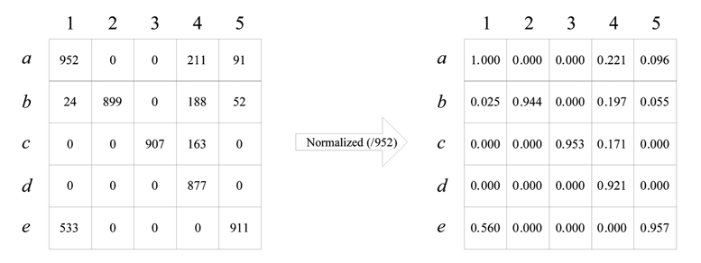
Based on the definition above, we can see that each query corresponds to an appearance sequence that embodies the reading habit of people, and the default rules of some industry, as mentioned in Section I. Now, the first task of our approach is turned into collecting the statistics about the positions of attributes in the appearance sequence. First of all, each query in the query log including only three types of queries (SPJ, SPJU, SPJS) is scanned, to produce an appearance sequence. The position of each attribute in an appearance sequence is recorded in a matrix. The row of the matrix represents all the attributes in one schema, while the column represents the positions from 1, to the maximum of the number of elements in all the appearance sequences. An entry of the matrix represents the number of some attribute appearing in some position in all the appearance sequences. This is our first type of matrix, and we call it a p-matrix. Before scanning the query log, all the entries in the p-matrix are initialized with the value 0. If an attribute appears in some position, the value of the corresponding entry in the p-matrix is incremented by one. After scanning all the queries in the query log, the entries in the p-matrix are normalized, by dividing each of them by the largest number of all entry numbers. After this normalization step, the p-matrix is independent of the size of the query log. To understand the p-matrix intuitively, an example with dummy statistics and six dummy attributes a – e is shown in the left-hand panel of Fig. 2, while the normalized one is shown in the other side.
Consider two appearance sequences, S1 = a1a2a3a4a5 and S2 = b1b2. Although the two attributes a1 and b1 are both in first position, we believe that a1 is greater than b1 in terms of the importance of structuring the query results to be shown to the final users. This is because a1 ranks prior to four attributes in its sequence, however, b1 ranks prior to only one attribute. As a result, it is not reasonable that attribute a1 is matched to attribute b1, with respect to the importance of attributes in the sequence. We can see that just the statistics about the positions of attributes in the sequence are not enough to discover the matches. As a result, we make a minor change to the original matrix, to collect the information about the number of attributes that rank after a given attribute in the appearance sequence. The changed matrix is called an n-matrix, which is our second type of matrix. Actually, the n-matrix is similar to the p-matrix, and they have the same columns and same rows. The difference between them is that each time the value of the corresponding entry for an attribute e increases, the increment is not the value 1, but rather the number of the attributes that rank after e in the appearance sequence. Except the information about the posipositions of attributes, the n-matrix captures a little more information than the p-matrix, and their performance is tested and compared in our experiment. The advantage of the n-matrix is that it considers not only the absolute positions of attributes, but also their relative positions, and this makes the importance of attributes in the sequences more general. Now, given two schemas to be matched, we can obtain two corresponding matrices. The two matrices can be seen as the respective feature of attributes in the two schemas. Thus, our task of matching attributes is transformed into measuring the similarity of the two matrices. In the next section, two scoring functions are introduced for the measurement of the similarity of the two matrices.
In this section, our discussion is divided into two parts. Two scoring functions are discussed in the first subsection, while the search algorithm is discussed in the second subsection.
Before the main discussion, we introduce several types of cardinality constraints in schema matching, which are the prerequisite of the scoring functions. The cardinality constraint is an important feature of the ER-diagram in the database. The constraints usually state instructions of the form “every person has exactly one mother”, or “every course must have at least one teacher”. They are very useful, because they allow the logical integrity of the database to be maintained. The cardinality constraints in schema matching are similar to the one in the database. Given two sets of attributes, the cardinality constraints state how many attributes in one set should hold correspondences with attributes in the other set. Thus, given a mapping, these constraints play an important role in the behavior of a scoring function. We will analyze the effect of these constraints on the scoring function in detail, in the remainder of this section. In our approach, we consider three types of cardinality constraints: one-to-one mapping, onto mapping, and partial mapping, which are first proposed in [2]. For two input schemas S1 and S2 to be matched, the three types of cardinality constraints are described as follows:
1) One-to-one mapping: For each attribute in S1, there exists one and only one corresponding attribute as the counterpart in S2, and vice versa. If the two schemas S1 and S2 are referred to as two sets and the mapping is referred to as a function, we can see that this function is the so-called bijective mapping in discrete mathematics, i.e., it is both surjection and incidence.2) Onto mapping: For each attribute in S1, there exists a unique attribute in S2 as a match. Conversely, each attribute in S2 either has one and only one attribute in S1 as a match, or remains unmatched. Compared to the one-to-one mapping, this mapping actually falls into the class of incidence.3) Partial mapping: Each attribute in S1 either has one and only one attribute in S2 as a match, or remains unmatched, and vice versa. In practice, this case is the most general and difficult one. The reason is that for an attribute in one schema, the existence of its match (counterpart) in another schema is unknown (uncertain); for a schema, the number of its attributes that have matches in another schema is unknown.
These three types of cardinality constraints are very prevalent in practice, as opposed to the case where an attribute in one schema has multiple matches in another schema, so in the proposed approach we do not consider this kind of cardinality constraint.
In essence, a scoring function is a function that takes some parameters of some entity, or some quantitative features of some model or some procedure as input, and then outputs a final numeric value (score), as a measurement of inputs. It is also a mapping from a set of parameters to a final numeric value. It is a computation rule, which embodies some measurements about what is good or bad, between inputs and the final score. The computation rule is the important component of the scoring function, because a set of appropriate rules is the key to obtaining an accurate final score. The problem of how to create an effective scoring function to evaluate the quality of matching has been discussed in [2]. They proposed two scoring functions, and addressed the problem of the monotonicity of scoring functions. They classified their scoring functions into monotonic and non-monotonic. Given the mapping, we exploit their scoring functions as the measurement of similarity of feature matrices in our approach. As in [5], we introduce some formal descriptions about schema matching. Let S1 and S2 be two schemas to be matched. Given their respective feature matrices, the matching task is to find the optimal mapping that gives the highest score for a specific scoring function. Consequently, any mapping m should provide three kinds of information for the scoring function. The first is the number of matches (matched attributes) included in m, denoted as km; the second is the attributes occurring in m, denoted as {a1, ..., ai, ..., akm} for S1 and {b1, ..., bj, ..., bkm} for S2; and the third is the actual correspondences between attributes of S1 and S2, i.e., m(ai) = bj (m(i) = j). Here, it should be noted that km is the number of matches in m, rather than the number of correct matches in m. For two feature matrices, they are required to have the same number of rows and columns for the computation of similarity. Thus, if the number of their rows and columns is not equal, additional rows and columns with values 0 are added to the end of the corresponding matrix. Now, we present the definition of the monotonic scoring function.
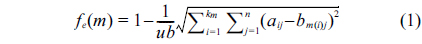
DEFINITION 2.LetP1 and P2be the two feature matrices collected from the query logs of schemaS1 and S2, respectively, and n be the number of the rows ofP1andP2. Let aij be an entry inP1, which represents the statistics about attribute ai appearing in position j, while bij is an entry inP2, which represents the statistics about attribute bi appearing in position j. Given a mapping m, the monotonic scoring function is defined as:
Given the mapping m, this scoring function employs the Euclidean distance metric to measure the similarity between two feature matrices. Let dm(P1, P2) be the Euclidean distance above, i.e., the square root item. We can see that dm(P1, P2) increases monotonically with the increase of the number of matches in m; that is, this function is monotonic in km. For example, let m1 = (a1, b1), m2 = (a1a2, b1b2) be two mappings. If n is set to 2, then dm1(P1, P2) is (a1 – b1)2, and dm2(P1, P2) is (a1 − b1)2 + (a2 − b2)2. As a result, dm2 is equal to or greater than dm1, because of (a2 − b2)2 ≥ 0; that is, the score decreases monotonically with the increase of km. Given two schemas to be matched, if the correct km is unknown, the matching algorithm using this function will just return the mapping with only one match as , because the score of any mapping with more than one match will be smaller than the one with only one match. As a result, this function can be used to achieve the one-to-one mapping and the onto mapping problems where the km is known, and as the input of search algorithms, rather than the partial mapping problem. The variable ub takes the value that is the upper bound to the value of dm(P1, P2); and this guarantees that the value of the function is positive. In the following, we will discuss the non-monotonic scoring function.
DEFINITION 3.LetP1andP2be the two feature matrices with n rows. Let aij be an entry inP1, which represents the statistics about attribute ai appearing in position j, whilebijis an entry inP2, which represents the statistics about attributebiappearing in position j. Given a mapping m, the non-monotonic scoring function is defined as:
This is a non-monotonic scoring function; that is, there is no monotonic relation between the score and the number km of matches in the mapping. Now, we will analyze the principle of this scoring function. The item multiplied by α in the equation above is the normal distance[2]. Suppose that, if the statistics values about the position of attributes are uniformly distributed, and two of them are randomly chosen from the matrices, the expected value of normal distance is β (around 1/3). As a result, if the control parameter α is set to 1/β (around 3), the expected score of this function becomes 0 with the assumption above. In other words, in such cases, the match of two randomly chosen attributes will not contribute to the final score. In contrast, if the match is correct (the two attributes map correctly), it will positively contribute to the final score. It can be seen that for a mapping m, the more correct matches m includes, the higher score m that is rewarded. Thus, the optimal mapping is expected to be rewarded with the highest score among other mappings. Based on the analysis above, we can see that this function is non-monotonic in km. For a search algorithm using the scoring function, the with the highest score is close to the ideal solution with much higher possibility. Consequently, the corresponding search algorithm can apply to all three kinds of mappings. We compare the two scoring functions over these mappings in our experiments. Actually, the value 1/α represents the average of the normal distance, or the approximate demarcation point between the normal distance of the correct matches, and the normal distance of the wrong matches. The control α can be computed via the quantile, or the experiments. Further, the behavior of the scoring function can be controlled, by changing the parameter α (see [2] for more details).
Given the feature matrices and the scoring functions, our task now is to find the optimal attribute mapping, namely the mapping with the highest score. In this section, we first introduce how to refer to the problem of searching the optimal mapping as a combinatorial optimization problem, then present the details of the search algorithm.
Given two schemas S1 and S2 to be matched, the first schema S1 has n1 attributes {a1, ..., ai, ..., an1}, while S2 has n2 attributes {b1, ..., bj, ..., bn2}. Consider the first cardinality constraint one-to-one mapping, where n1 = n2. If the attributes of S1 are regarded as a fixed sequence a1a2 ...an1 and the correspondence is fixed m(ai) = bi, any instance of the permutation of all attributes of S2 corresponds to a possible mapping. For example, if n1 = n2 = 2, then the permutation b1b2 and b2b1 correspond to two possible mappings {(a1, b1), (a2, b2)} and {(a1, b2), (a2, b1)}, where each mapping includes two matches. As a result, we can see that our task of finding the can be transformed into a combinatorial optimization problem, where the score of each permutation is the score of its corresponding mapping. However, for the other two cardinality constraints of onto mapping and partial mapping, the numbers of the attributes of the two schemas are typically not equal. To perform the problem transformation above, we need to make the two schemas own the same number of attributes n. For this purpose, the ‘dummy’ attributes [5] are added to S1 and S2. The problem of how many attributes should be added depends on the scoring function. If the monotonic function is used, then n2 − attributes will be added to S1, while n1 − attributes will be added to S2, so each schema has n1 + n2 − = n attributes. Here, for onto mapping, is also known, and takes the value min(n1, n2); but for partial mapping, it is the estimate of the number of the correct matches between S1 and S2, and should be given to the algorithm. Now, we describe how to decide the number of attributes that are added. For S2, there exist n2 − attributes {bq...br} that have no matching attributes in S1, so n2 − ‘dummy’ attributes are added to S1 as the matching attributes for {bq...br}. The reason for S1 is the same as S2; thus we will no longer give unnecessary details. For the non-monotonic function, the is not required, so it is considered to be zero. Thus, n2 ‘dummy’ attribute will be added to S1, while n1 ‘dummy’ attributes will be added to S2. We can see that in addition to making the two schemas have the same number of attributes, another purpose of the ‘dummy’ attributes is to make each attribute have a counterpart in the other schema. In addition, the ‘dummy’ attribute enables the feature marices to have the same number of rows with value 0. So, we only need to add some columns into the feature matrices to make them have the same size. Here, it should be noted that, when the search algorithm computes the score of a mapping, the matches that involve the ‘dummy’ attributes are ignored.
Next, we will discuss the search algorithm. We can see that while regarding the attributes of S1 as a fixed sequence, the number of the permutations of all attributes of S2 is n!. The space of all the permutations is very large, and an exhaustive search is not feasible. Thus, we exploit the simulated annealing (SA) algorithm [6], which is the classical solution to the combinatorial optimization problem, to find the optimal permutation corresponding to , denoted by . SA algorithm is a random search technique based on the physical annealing process, which can gradually approach global optimization, by continuously breaking off from local optimization. SA is a generic probabilistic metaheuristic for the global optimization problem in a large search space. It is fit for a search space that is discrete. For certain problems, SA may be more efficient than an exhaustive search, if the globally optimal solution is not necessary for users. The inspiration of SA is from annealing in metallurgy, which is a technique involving the heating and controlled cooling of a material, to increase the size of its crystals, and to reduce their defects. The energy function of SA represents the energy of the solids that are heated. In our context, the scoring functions are used as the energy function of SA. It should be noted that we aim at the solution with the highest score, rather than the usual lowest energy. The SA algorithm involves six key components: the generator of new solutions, the Metropolis criterion, the initial temperature, the length of Markov chain, the temperature-fall period, and the stopping criteria. We now briefly explain each of these components in our context.
The purpose of the first component is to explore the solutions in the search space. The generator should uniformly explore the space, which benefits the discovery of global optimization. There are many methods that can be used as the solution generator, for example, the methods from the genetic algorithm. The implementation of our generator is shown in Algorithm 1. The main idea of the algorithm is to use some ordering and exchanging rules based on two random numbers, to generate the new solutions. Given a current solution b1b2…bn, two numbers q and r are randomly generated. If q > r, the elements from bq to br are re-arranged in reverse order, while the order of other elements remains unchanged. If q > r, the elements from b1 to br and from bq to bn are conversely rearranged, respectively. If q = r, the elements from b1 to bq are conversely re-arranged. Here, other methods can also be used, for example the cross and mutation leveraged from the genetic algorithm.
The Metropolis criterion represents the acceptance criterion of the new solutions. We use an example to explain this criterion. Let p1 be the current solution, p2 be the new solution, and f(x) be the scoring function, i.e., fe(x) or fn(x). The Metropolis criterion means that if f(p2) > f(p1), use p2 as the current solution instead of p1; else if exp > rn , also accept p2; else preserve p1 and abandon p2, where rn is a random number in the range (0,1), and T is the current temperature. When the score of the new solution is greater than the current solution (f(p2) > f(p1)), then we accept the new solution, and make a small forward step towards global optimization. When the score of the new solution is less than the current solution, the algorithm will accept the new solution with some probabilities. This step can guarantee that the algorithm can break from the local optimization with some probabilities, and approach the global optimization gradually. SA algorithm makes use of this criterion, to make a decision about whether or not to accept the new solutions.
The initial temperature T0 of SA is central to obtaining the global optimization, and the higher T0 is, the closer the solutions approach the real solution. However, a much higher T0 will lead to a large number of loops, which will result in a unacceptable running time, namely a very slow convergence speed. Kirkpatrick and Vecchi [6] proposed that T0 should enable the acceptance rate of new solutions to approach the value 1 at the beginning. This means that the acceptance possibility of Metropolis criterion is close to 1 at the beginning, i.e., exp . To obtain more accurate solution and relatively less running time, this possibility is typically set to 0.95 in practice. To use this method to compute T0 in our context, we need to compute Δ>f>. Here, the statistical method is used to compute the score dif>f>e>>rence. We randomly choose k pairs of solutions (k > 1000), then compute the score dif>f>e>>rence of each pair, and finally, take the expectation of these dif>f>e>>rences as the value of Δ>f>.
The last three components of SA are relatively simple. The length of the Markov chain refers to the number of iterations traversing the new solutions under a certain temperature. Intuitively, the longer the length is, the more accurate the solution is. However, the length is topically associated with the problem size, and overly long chains would not help find global optimization [6]. Thus, the length of Markov chain in our approach is set to 10n. For the temperature-fall period, we make use of the classical method, i.e., Tk+1 = βTk, to control the attenuation of the temperature, where β = 0.95, and Tk is the current temperature. In theory, we can obtain a more accurate solution using a higher β. However, a higher β will lead to an unacceptable running time. During the running of the algorithm, if consecutive r Markov chains have no improvement on the current optimization, the search process will terminate; this is the stopping criterion. Now, based on these components, the details of the search algorithm are shown in Algorithm 2.
The algorithm begins with a random solution (line 1), because the initial solution has very little effect on its performance. Then, it randomly explores the new solutions (line 5), and employs the Metropolis criterion, to decide whether to update the current solution (lines 6–11). Actually, the internal loop corresponds to a Markov chain (lines 4–13), where line 13 is the length of the Markov chain.
Thus, each iteration of the external loop will generate a Markov chain. If the length exceeds 10n, the spread of the chain is over (line 13), and the temperature falls for the next chain (line 14). If after r iterations of the external loop the current solution remains unchanged, the algorithm will terminate, and return the current solution as .
In this section, we test the time cost, and evaluate the quality of the matching results of our proposed approach, in synthetic schema matching scenarios. First, we present how to generate the synthetic data set used in the experiments. Then, we show the experimental results evaluating the performance of our matching algorithm, in the case of the three cardinality constraints (one-to-one, onto, and partial). We also study the effect of varying the control parameter of the non-monotonic function on the performance of our approach. Finally, we test the time cost of the proposed algorithm. Our algorithm is implemented using C++ language, and the experiments are carried on a PC compatible machine, with Intel Core Duo processor (2.33 GHz).
We generate the experimental data set based on two online bookstores developed by different persons. The schema of the first bookstore includes 31 attributes, while the second includes 35 attributes, and there exist 27 matching attributes (matches) of each schema. We suppose that a fictitious user continuously accesses each bookstore, until the produced log includes 8000 queries. These SQL statements include two kinds of queries: random queries with any keywords, according to the query interface of the bookstore; and fixed queries, generated based on the navigation or classification functions of the bookstore. The first kind of queries mainly makes use of schema attributes as query criteria to find books. The attributes used include ‘bookName’, ‘author’, ‘publisher’, and ‘pubtime’, where the rest of the attributes are not considered, because of their lower frequency of use. The first kinds of queries are also divided into four parts, each of which has a different attribute as a query criterion. We assign different percentages to the queries with different attributes, according to their use frequency. That is, we generate 40% queries using the attribute ‘bookName’, 30% query using ‘author’, 20% queries using ‘publisher’, and 10% queries using ‘pubtime’. We simulate the actual case by this method. Based on the query logs, the two feature matrices of the bookstores can be obtained as the experimental data. In the experiments, the F-Measure metrics are used as the measurement of the performance of the algorithm.
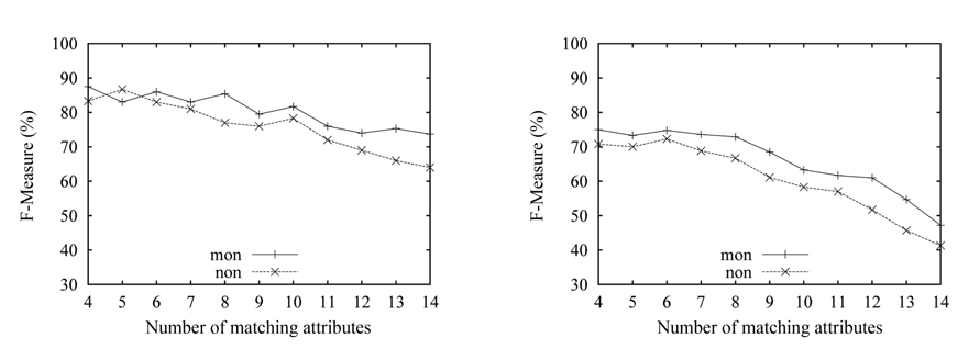
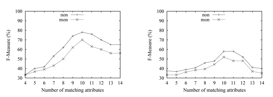
We evaluate the accuracy against the correct mappings determined by manual inspection of the source and target schemas. We run our algorithm with randomly chosen subsets of the experimental data in each experiment for many times, then get the average of the experimental results. We first present the results of one-to-one mapping in Fig. 3. We use the notation ‘mon’ and ‘non’ as shorthand for the monotonic function and the non-monotonic function, respectively. The control parameter α for the non-monotonic function is set to 0.3.
As can be seen in Fig. 3(a), the match results gradually deteriorate, as the number of the matching attributes (matches) increases, and the worst result for the ‘non’ function is nearly 60%. The changing trends of the two curves are almost the same, namely decreasing with the increase of the number of matches. It is obvious that the accuracy will decrease with the increase of matches, because the increase of the number of matching attributes will result in the increase of the space of the candidate matches. The results with ‘mon’ are better than the one with ‘non’. This is because the correct km is known for the one-to-one mapping. We can also see that the overall quality of the results over the n-matrix is higher, than the one over the p-matrix. The reason is that the information collected in the n-matrix is more than the information in the p-matrix, and this behavior conforms to our theoretical analysis in the section above.
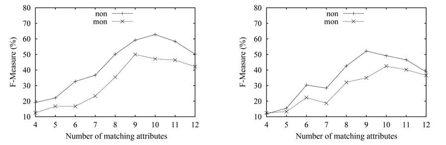
The experimental results corresponding to the onto cardinality constraint are shown in Fig. 4. Here, the size of the target schema is kept constant at 16 attributes,while the matching attribute number of the source schema is increased from 4 to 14. As can be seen in both data sets, the results with ‘non’ outperform the results with ‘mon’. The accuracy with ‘non’ reaches 80% in Fig. 4(a), while it was 59% in Fig. 4(b). It can be seen that the ‘non’ scoring function shows its advantage, compared to the ‘mon’ scoring function, when the real km is unknown. The overall quality over the n-matrix is better than over the p-matrix. The changing trends of curves here are different from the one in Fig. 3. The accuracy in the onto mapping case gradually improves, as the number of matching attributes increases; then the accuracy begins to decline, when the number exceeds some value; this is just contrary to the one-to-one mapping. The reason is that the matching with the onto constraint requires extra effort, in contrast to the one-to-one case, i.e., the onto mapping first needs to choose a subset of the 16 attributes as the matching attributes that will participate in the following matching process, then the onto mapping based on the chosen attribute subset is turned into the one-to-one mapping. At the beginning, the space of the attribute subsets is very large, because of the lesser attributes of the source schema. Thus, the accuracy is low, and the lowest is around 30%. With the increase of the attributes of the source schema, the accuracy gradually rises.
Fig. 5 illustrates the results of the matching with the partial mapping cardinality constraint. In this experiment, we fix the size of both source and target schema at 14, and vary the number of the matching attributes from 4 to 12. To enable the experiment with the ‘mon’ in the partial mapping case, we give the number of the correct matches to the algorithm with the ‘mon’ function. When the number of matching attributes is less than 5, the accuracy is very low, under 15%. Thus, the results when the attribute number is under 4 are not shown in Fig. 4. Here, the trend of curves in Fig. 5 is similar to the above experiment, but the best performance is less than 70%. The reason is that the matching process with partial cardinality is similar to the one with onto cardinality, namely the algorithm needs to choose a subset of the attributes from the attribute universe. Thus, the accuracy is very low, when the matching attributes involved in the matching process are less. That is, the search space is very large, when the matching attribute number is few. It can be seen that the matching with the partial cardinality constraint is the most difficult matching. Conversely, the results with the ‘non’ function are better, than the one with the ‘mon’ function.
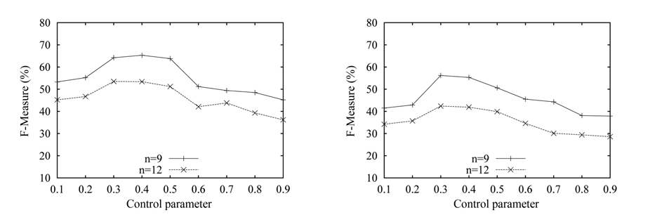
Now, we test the effect of varying the control parameter α on the match results. We fix the size of both source and target schema at 14 attributes, and fix the number of the correct matches at 9 and 12, respectively, denoted by n = 12 and n = 9. The experimental results are shown in Fig. 6. We can see that the accuracy first increases, as α increases from 0.1 to 0.3; then achieves the highest value as α ∈ (0.3, 0.5); and finally drops, with the increase of α. When α is under 0.3, most of the true matches are punished with negative score. Conversely, lots of false matches are rewarded with positive score. Thus, at the beginning, the accuracy is low. With α approaching the value ‘0.3’, the accuracy gradually reaches the greatest value, of around 70%. Then, the accuracy gradually declines, because of the punishment of most of the matches. The accuracy with n = 9 is higher than the one with n = 12, and the results over the n-matrix are better than those over the pmatrix, which is consistent with the above experiments.
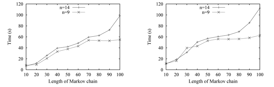
Finally, we test the time cost of our algorithm with one-to-one cardinality constraint, and α is also set to 0.3. In this experiment, we set the number of the correct matches to 9 and 14, respectively, denoted by n = 9 and n = 14, and set the temperature-fall coefficient β = 0.9 and β = 0.95. The y-coordinate represents time cost, while the x-coordinate represents the length of Markov chain. The results are shown in Fig. 7. The time with n =14 increases, as the length of the Markov chain increases; and the longest running time reaches nearly two minutes. Obviously, the time cost increases, because of the iterations caused by the increase of the length of Markov chain. However, the time cost with n = 9 remains unchanged, after a length beyond 60. The reason for this behavior is that the size of the search space for n = 9 is less than the number of all iterations of the algorithm, so the algorithm will accomplish the search process ahead of time, and ignore the following iterations caused by the increase of length. It can also be seen that the time cost for β = 0.9 in Fig. 7(a) is less than the cost for β = 0.95 in Fig. 7(b). The reason is that the number of iterations increases for β = 0.95.
참고문헌
1.
Rahm E., Bernstein P. A.
2001
“A survey of approaches to automatic schema matching,”
[VLDB Journal]
Vol.10 P.334-350
2.
Kang J., Naughton J. F.
2003
“On schema matching with opaque column names and data values,”
[in Proceedings of the 2003 ACM SIGMOD International Conference on Management of Data]
P.205-216
3.
Madhavan J., Bernstein P. A., Doan A., Halevy A.
2005
“Corpus-based schema matching,”
[in Proceedings of the 21st International Conference on Data Engineering]
P.57-68
4.
Dong X., Halevy A. Y., Yu C.
2007
“Data integration with uncertainty,”
[in Proceedings of the 33rd International Conference on Very Large Data Bases]
P.687-698
5.
Elmeleegy H., Ouzzani M., Elmagarmid A.
2008
“Usagebased schema matching,”
[in Proceedings of the 24th International Conference on Data Engineering]
P.20-29
6.
Kirkpatrick S., Vecchi M. P.
1983
“Optimization by simmulated annealing,”
[Science]
Vol.220 P.671-680
7.
Bohannon P., Elnahrawy E., Fan W., Flaster M.
2006
“Putting context into schema matching,”
[in Proceedings of the 32nd International Conference on Very Large Data Bases]
P.307-318
8.
Popa L., Velegrakis Y., Hernandez M. A., Miller R. J., Fagin R.
2002
“Translating web data,”
[in Proceedings of the 28th International Conference on Very Large Data Bases]
P.598-609
9.
Miller R. J., Haas L. M., Hernandez M. A.
2000
“Schema mapping as query discovery,”
[in Proceedings of the 26th International Conference on Very Large Data Bases]
P.77-88
10.
An Y., Borgida A., Miller R. J., Mylopoulos J.
2007
“A semantic approach to discovering schema mapping expressions,”
[in Proceedings of the 23rd International Conference on Data Engineering]
P.206-215
11.
Mecca G., Papotti P., Raunich S.
2009
“Core schema mappings,”
[in Proceedings of the ACM SIGMOD International Conference on Management of Data]
P.655-668
12.
Melnik S., Garcia-Molina H., Rahm E.
2002
“Similarity flooding: a versatile graph matching algorithm and its application to schema matching,”
[in Proceedings of the 18th International Conference on Data Engineering]
P.117-128
13.
Das Sarma A., Dong X., Halevy A.
2008
“Bootstrapping pay-as-you-go data integration systems,”
[in Proceedings of the ACM SIGMOD International Conference on Management of Data]
P.861-874
14.
Fagin R., Kolaitis P. G., Miller R. J., Popa L.
2003
“Data exchange: semantics and query answering,”
[in Proceedings of the 9th International Conference on Database Theory]
P.207-224
15.
Warren R. H., Tompa F. W.
2006
“Multi-column substring matching for database schema translation,”
[in Proceedings of the 32nd International Conference on Very Large Data Bases]
P.331-342
OAK XML 통계
이미지 / 테이블
[
Fig. 1.
]
Schema structure of query results from five digital libraries A-E.