A symplectic integration method is a numerical method for solving Hamiltonian equations,

a special class of differential equations related to classical mechanics and symplectic geometry. Various symplectic methods are designed and widely used in celestial mechanics, molecular dynamics, electromagnetic field analysis, etc., particularly for the longterm integration of Hamiltonian equations.

The time evolution of Hamiltonian equations preserves a special differential 2-form dp∧dq called the symplectic form. A numerical method is said to be symplectic if it also preserves the symplectic form. Since the concept of symplectic integration methods was proposed in the mid- 1980s [1], many mathematical researches have been carried out [2-4]. In particular, it has been revealed that a symplectic method preserves an approximate Hamiltonian perturbed from the original Hamiltonian [5, 6]. It theoretically supports the effectiveness of symplectic methods for long-term integration.

On the other hand, the numerical stability of symplectic methods has received little attention, although it is also related to long-term integration; only a few papers [7, 8] deal with this subject. It is certain that many outstanding symplectic methods are implicit and possess originally superior stability. However, in a large-scale computation, e.g., in the solution of partial differential equations, explicit methods are still effective tools. A study of their stability has significance for practical computation because the stability of numerical methods is closely related to step size restrictions, such as a Courant-Friedrichs-Lewy (CFL) condition for hyperbolic equations.

In this paper, we study the stability of an explicit symplectic method by using the harmonic oscillator as a test equation, following [8]. An outline of this paper is as follows: In Section II, we describe the fundamental concept and notation concerning explicit symplectic methods and their numerical stability. In Section III, we propose a new stability criterion for the symplectic methods and discuss the stability of the basic methods on the basis of this criterion. In Section IV, we continue to analyze more advanced methods and derive a new method, which is tested through a numerical experiment with the sine-Gordon equation, a nonlinear wave equa-tion in Section V.

We consider a Hamiltonian of the special form

and the initial value problem

for the corresponding Hamiltonian equation, where

In mechanics, T and U represent kinetic energy and potential energy, respectively.

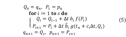
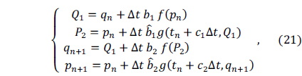
In general, symplectic methods are implicit; i.e., it is necessary to solve nonlinear equations for the implementation of these methods. For problem (3), there are explicit symplectic methods by virtue of the special form (2). A well-known instance is a symplectic partitioned Runge-Kutta method, whose general form is as follows (see, e.g., [2, 4]):

Here, Δt > 0 is the time step size, t_n = nΔt(n = 0,1,… ), and q_n p_n are approximate values for q(t_n) and p(t_n) , respectively. Further, b₁, b₂, … b_s, and are parameters of the method, and Q_i and P_i are intermediate variables for computation. The parameters of the method, determined from order conditions [2, 4], are often written as

To study the stability of the symplectic method (5), we adopt the harmonic oscillator

as a test equation ([8]; see also [7] for another test equation). This is a Hamiltonian equation with the Hamiltonian H(p,q) = (ω /2 )(p²+q²), ω ≥ 0. We also adopt the scaled step size

as a basic parameter for the stability analysis. Upon the restriction of the frequency ω ≥ 0, the range of the parameter is θ ≥ 0.

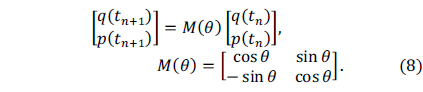
It should be noted that exact solutions to (6) satisfy

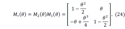
The matrix M(≥) is an orthogonal matrix, and its eigenvalues are , both of which have unit modulus.

In the case f(p) = ωp and g(t,q) = −ωq, the equations for the intermediate variables in (5) becomes

The substitution of the first equation into the second equation gives Hence, (9) is rewritten as

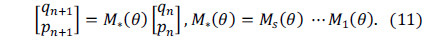
and application of method (5) to test equation (6) yields an analogue to (8),

It is clear that det M_i(θ) = 1. Hence M_*(θ) = 1 holds for any method of the form(5). The Characteristic equation M_*(θ) is written as

and the eigen values are given by

where tr M_*(θ) denotes the trace of the matrix M_*(θ). If │ tr M_*(θ)│ < 2, the eigenvalues are complex numbers with |λ|=1. If tr M_*(θ) = 2, then λ = 1, and if tr M_*(θ) = − 2, then λ = − 1. If │tr M_*(θ)│ > 2, the eigenvalues are real, and one of them satisfies |λ| > 1. The set {θ ≥ 0 : │ tr M_*(θ)│ ≤ 2} is a union of closed intervals. The connected component of the set that contains the origin is called the stability interval of method (5), which has been used for comparing the stability of numerical methods [8].

If │tr M_*(θ)│ < 2, M_*(θ) has complex conjugate eigenvalues λ, which satisfy │λ│=││= 1 and λ ≠ Hence, M_*(θ) is represented in form

with some nonsingular matrix T. Since

and │λ│=││ = 1, we have ║M_*(θ)ⁿ║ ≤║T║ ║T^-1║ for any integer n ≥ 0, where ║•║ denotes the matrix norm induced from the Euclidean norm. The upper bound ║T║║T^-1║ is represented as follows.

Theorem 1. Let a,b,c,d be real numbers, Assume that satisfies det M = 1 and │ tr M│ < 2. Then, we have

for any integer n ≥ 0, where

The proof of the theorem is obtained by a simple but tiresome computation. We omit the proof (cf. the proof of Theorem 3.1 in [9]). As shown below, ϕ in Theorem 1 is used as a criterion for the stability of the numerical methods.

In the case s = 1 and (5) is reducde to

This is called the symplectic Euler method and is of the order 1 in accuracy. In the case of the symplectic Euler method, we have

Since tr M(θ) = 2 - θ², the stability interval of the method is [0, 2]. For 0 < θ < 2, ϕ in Theorem 1 is computed as

In the case s = 2, method (5) is rewritten as

which is of the order 2 if the parameters satisfy

In particular, the parameter values

satisfy the condition, and the corresponding method is known as the Störmer - Verlet method [4, 8].

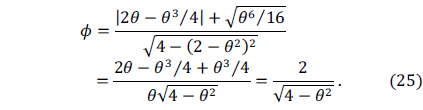
For this method, we have

Since tr M(θ) = 2 − θ², the stability interval of the Stormer - Verlet method is [0, 2], which is the same as that of the symplectic Euler method. However, since (2θ - θ³/4)² - {4 - (2 - θ²)²} = θ⁶/16 , we have, for 0 < θ < 2,

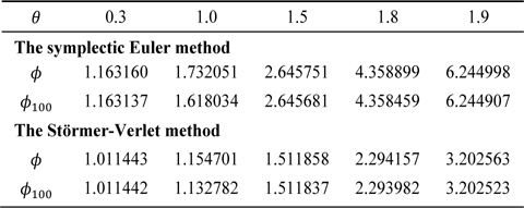
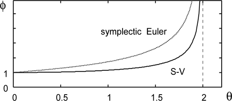
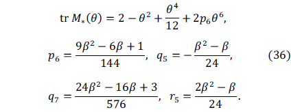
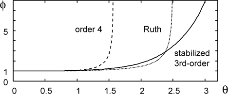
Fig. 1 shows the functions ϕ for the two methods. Function (25) for the Störmer-Verlet method is closer to the line ϕ = 1 than (20) for the symplectic Euler method. The matrix M ( θ ) in (8) is an orthogonal matrix and satisfies ║M(θ)ⁿ║ = 1 for any θ ≥ 0 and any integer n ≥ 0. Since (25) reflects this property more appropriately than (20), we can consider the Störmer-Verlet method has a better stability property than the symplectic Euler method although the two methods have the same stability intervals.

Table 1 presents ϕ and ϕ ₁₀₀ = max _{0≤n ≤100}║M_*(θ)ⁿ║, computed numerically, for several values of θ . This shows that ϕ gives an appropriate approximation to sup_n≥0 ║M_*(θ)ⁿ║ except θ = 1

Method (5) for s = 3 corresponding to the parameter values

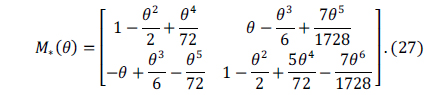
is called Ruth’s method, which is of the order 3 in accuracy. For Ruth’s method, we have

The stability interval is ≈2.50748 where denotes a root of tr M_*(θ) = −2.

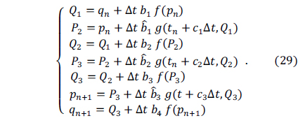
To try to improve Ruth’s method with respect to stability, we consider (5) for s = 4 with , which is reduced to

At first glance, it appears that (29) needs more evaluation of f than (5) with s = 3, but f(p_n+1) for the computation of q_n+1 is again used for the computation of Q₁ at the next step t = t_n+1. Hence, from the perspective of function evaluation, the work needed for (29) is the same as that for (5) with s = 3 e. g., Ruth’s method. This idea is called first same as last and is often utilized in the numerical analysis of differential equations [2].

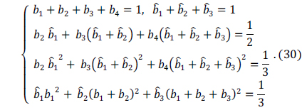
Method (29) is of the order 3 if the parameters satisfy

These are too complicated to treat. We thus introduce the simplifying condition

By virtue of this condition, the coefficient of θ⁶ in tr M_*(θ) becomes 0, and the trace is reduced to

The stability interval becomes which is larger than that of Ruth’s method.

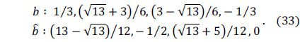
Eqs. (30) and (31) form a system of 6 equations with 7 unknown variables, which has solutions with a free parameter, e.g., b₁. Letting b₁ = 1/3, we obtain the following :

We refer to the corresponding method as the stabilized 3rd-order method. In Fig. 2, the functions ϕ for Ruth’s method and the stabilized 3rd-order method are presented. For θ ≤ 2.37, ϕ for Ruth’s method is smaller than ϕ for the stabilized 3rd-order method, but the latter has finite values up to

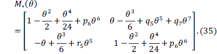
Several symplectic methods of the order 4 are known. Among them, a method of the form (29) corresponding to the parameter values (see, e.g., [4], p. 109)

For this method, we have the following:

The stability interval is ≈ 1.57340, where is a root of tr M_* (θ) = 2 . The stability interval is smaller than that of the symplectic Euler method (Fig. 2).

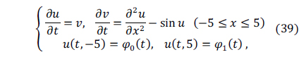
To test our numerical method, we consider the sine- Gordon equation

This equation has the solitary wave solution (see, e.g., [10], chapter 17).

By introducing a new variable v = 𝜕u/𝜕t and restricting the space variable x to -5 ≤ x≤ 5, we get the problem

where φ₀(t) and φ₁(t) are given so that (38) satisfies (39). Moreover, we apply the method of lines approximation to problem (39) by using a mesh of the form x_j = -5 + jΔ x, j = 0,1 …, M, Δx = 10/M, enotes a positive integer. As usual, we denote approximate functions to u(t,x_j) and v(t,x_j) by u_j(t) and v_j(t), respectively. By approximating 𝜕²u/𝜕x² with the standard central difference scheme, we get a Hamiltonian equation

where q(t) = [u₁(t), u₂(t), …, u_M-1(t)]^T, p(t) = [v₁(t), v₂(t), …, v_M-1(t)]^T

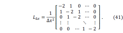
The matrix L_Δx has eigenvalues represented as

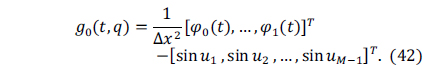
By using a linear transform, we change the linear part of (40) into equations of the form

Since ω_M-1 is the largest among ω_j’s, a symplectic method is stable for the linear part of (40) if ω_M-1 Δt is included in the interior of the stability interval. Denoting the stability interval by [0, θ₀] we express this condition as

which gives, M → ∞ a CFL condition

We now consider time step sizes of the form Δt = 10/N, where N is a positive integer, and assume 3N = 2M for M and N. Then, since Δt / Δx = 3/2, among the specific symplectic methods in Sections 2 and 3, only the stabilized 3rd-order method satisfies the CFL condition (46).

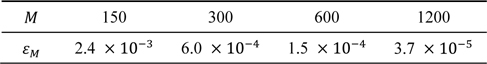
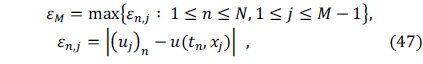
Table 2 shows the errors

for M = 150, 300, 600, 1200, in the case γ = 1 ⁄2 . It is observed that the numerical solution converges to the exact solution (38) with O (Δx²). For this selection of Δx and Δt, the other methods bring no significant numerical results because of overflow.