Processor architectural design has traditionally focused on improving average-case performance or energy efficiency. However, for real-time systems, time-predictability is the most important design consideration. Unfortunately, many performance-enhancing architectural features of today’s microprocessors, such as caches and branch predictions, are detrimental to time-predictability [1, 2]. As a result, an estimation of worst-case execution time (WCET) on modern microprocessors, which is crucial for hard real-time and safety-critical systems, is very difficult, if not impossible, to make [1, 2]. On the other hand, a time-predictable processor with low performance may be ineffective or even useless. To achieve both time-predictability and performance, researchers have proposed a time-predictable design for microprocessors [2] with the goal to achieve time-predictability (or WCET analyzeability) while minimizing the impact on average-case performance.

In the last two decades, researchers have proposed several designs of time-predictable processors for real-time systems. Colnaric and Halang [3] proposed a simple asymmetrical multiprocessor architecture without dynamic architectural features, such as pipelines and caches, for hard real-time applications. Delvai et al. [4] designed a scalable processor for embedded real-time applications, which employed a simple 3-stage pipeline without cache memory, and Edwards and Lee [5] proposed a precision timed (PRET) machine. Yamasaki et al. [6] studied instructions per cycle (IPC) control and prioritization of multithreaded processors. Paolieri et al. [7] examined time-predictable multicore architectures to support WCET analyzability. Finally, Schoeberl [8] proposed time-predictable Java processor.

However, to the best of our knowledge, none of the prior work has quantitatively evaluated time-predictability. While (average-case) performance can be easily assessed, most prior work on time-predictable design either simply reported the worst-case performance through measurement or analysis or just qualitatively explained that the design was time-predictable by removing undesirable architectural features. This is because, to the best of our knowledge, there is no well-defined metric to evaluate time-predictability of microprocessors, and this has fundamentally limited the advance of time-predictable architectural design. The lack of a metric does not only prevent designers from performing a quantitative comparison of different time-predictable designs in order to select the better one, but also makes it impossible to quantitatively analyze the trade-off between time-predictability and performance since these two goals often conflict with each other.

To address this problem, this paper proposes to use the standard deviation of cycles per instruction (CPI) to measure the time-predictability of different architectures. Such a metric can quantitatively indicate the variation in execution time of different architectural/microarchitectural designs, and thus can provide useful insights for engineers to make better design tradeoffs between performance and time-predictability.

The execution time of a real-time task (or generally a program) can be calculated by using Eq. (1), where T is the execution time, N is the number of instructions, CPI represents the clock cycles per instruction, and τ stands for the clock cycle time. The computer architecture community has used this equation to evaluate the average-case performance of microprocessors for decades, and we can also use it explain the variation of the execution time. In this equation, τ is fixed for each instruction, which is a predictable quantity after the processor is designed and implemented. In contrast, both N and CPI can vary significantly, thus making it hard to achieve time-predictability. Specifically, the number of instructions (N) can be affected by both software and instruction set architecture (ISA). Given an ISA, the number of instructions is mainly determined by the software and its inputs, i.e., which paths are executed at runtime. The CPI is affected by the architectural/microarchitectural design. Usually in a pipelined processor, different types of instructions take various clock cycles, and even the same type of instructions may take different clock cycles. For example, the latencies of load instructions depend on whether they hit in the cache or not.

[]

Since our goal is to design time-predictable processors (to support running real-time software), we should separate the time variation caused by software and hardware. For example, the inputs that are given, or the program paths that are executed, should not be a concern for hardware design. Prior work [2] seems to consider time-predictability of both the software and hardware as a single problem, making it overly complicated, if not impossible, to define a useful metric to specifically guide hardware design for time-predictability. In this paper, we propose a concept called architectural time-predictability (ATP) using the definition below.

Definition 1 (Architectural time-predictability). Given a number of instructions, architectural time-predictability indicates the degree that the architecture under study can provide predictable execution time.

In the above definition, the number of instructions of the ISA is assumed to be known, which we believe is a reasonable assumption to separate the time-predictability of software and hardware. Once the ISA is defined, the number of instructions executed is mostly affected by software characteristics, features, and processes, including the algorithm design, inputs, and compilation. Moreover, the number of instructions can be accurately obtained. For hard real-time systems, the worst-case number of instructions executed is needed to compute the WCET. The worst-case number of instructions can be calculated by state-of-the-art timing analysis techniques, such as the implicit path enumeration technique (IPET) [9], although the worst-case inputs may not be known without exhaustive measurements, which are prohibitive.

We propose to use the standard deviation of CPI to quantitatively evaluate architectural time-predictability. The averaged CPI has been used by the computer architecture community as a key measure of microarchitecture effectiveness. However, as an aggregate metric, it cannot indicate the variation of clock cycles for different instructions. As mentioned above, different instructions usually vary in the amount of clock cycles they take on modern processors, which is the fundamental reason why it is so difficult to predict microarchitectural timing during WCET analysis [1]. Therefore, we use the standard deviation of CPI, which can clearly indicate the amount of variation of microarchitectural timing, to measure architectural time-predictability. In the ideal scenarion, there is 100% time-predictability of the architecture (i.e., the standard deviation of CPI is 0), and it becomes trivial to compute the WCET. When we apply Eq. (1) to this ideal case, both CPI and τ are known, and the worst-case number of instructions is independent of hardware design and can be calculated by using today’s timing analysis techniques, such as IPET [9].

In modern processors, different types of instructions usually have different latencies. For example, an integer addition instruction is usually faster than a load instruction. Thus the standard deviation of CPI needs to be classified into the standard deviation of CPI for each type of instruction, rather than the standard deviation of CPI for all instructions. For instance, in a time-predictable processor, it is desirable for all the loads to take the same number of clock cycles. However, it would be unwise or unnecessary to require all loads to take the same amount of clock cycles as additions and subtractions. Thus in our evaluation, we classify the standard deviation for three types of instructions, including loads, stores, and other regular instructions.

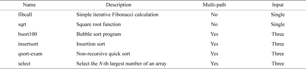
We simulate a superscalar processor with different architectural features to evaluate architectural time-predictability quantitatively based on the standard deviation of CPI, by using SimpleScalar, a cycle-accurate simulator [10]. We select six real-time benchmarks (Table 1) from the Malardalen WCET benchmark suite [11] for our experiments. Two of them are single-pathed, the other four have multiple paths, and each of them is executed with various inputs. We select three representative inputs to represent the best case, the normal case, and the worst case behavior observed (though it may not be the theoretical best/worst case).

[Table 1.] Real-time benchmarks used in our experiments

Real-time benchmarks used in our experiments

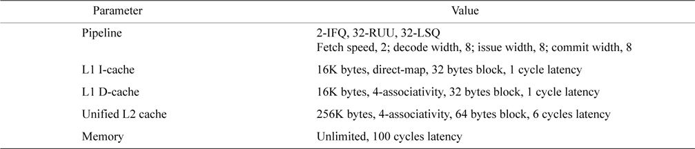
The basic configuration of the simulated processors is listed in Table 2, including the parameters of the pipelines, the caches, and the memory.

Caches and pipelines are two important architectural features that can boost performance and are widely employed in modern processors. Due to space limitations, our experiments in this paper focus on evaluating architectural time-predictability of caches and pipelines. More specifically, we quantitatively compare the architectural time-predictability of four different architectures with features as those given in Table 2.

With caches, with pipelines: a processor with L1 instruction cache, L1 data cache, L2 cache, and pipelines. With caches, without pipelines: a processor with L1 instruction cache, L1 data cache, and L2 cache, but no pipeline. Without caches, with pipelines: a processor with no cache and with pipelines. Without caches, without pipelines: a processor with no cache and no pipeline.

[Table 2.] Basic configuration of the simulated processor

Basic configuration of the simulated processor

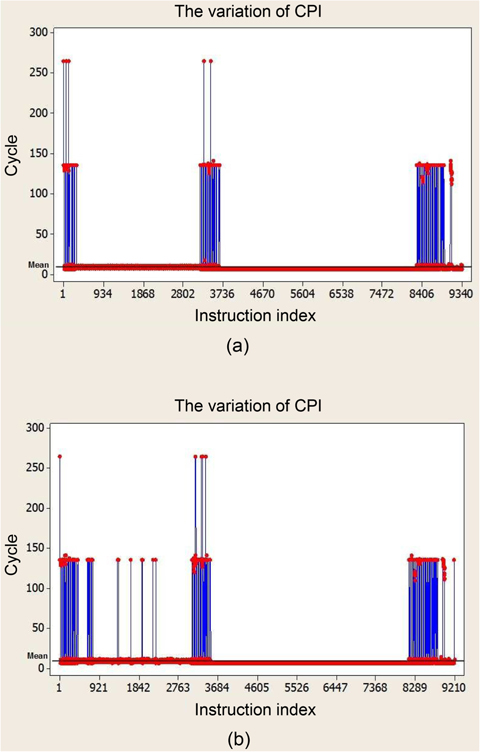
Our first experiment quantifies the variation of CPI for different benchmarks on a regular processor with caches and pipelines. Fig. 1 shows the variation of CPI of all the instructions for the benchmarks insertsort and qsortexam, both with the worst-case inputs. In the rest of the paper, all the experimental results are based on the worst-case inputs, whose timing behaviors are particularly important for hard real-time systems. The black line in each figure shows the mean CPI of all instructions of the benchmark. As we can see for both benchmarks, the CPIs vary significantly, indicating bad time-predictability of the default architecture (i.e., with caches and pipelines).

[Fig. 1.] The variation of cycles per instruction (CPI) of all the instructions for the benchmarks (a) insertsort and (b) qsort-exam both with the worst-case input.

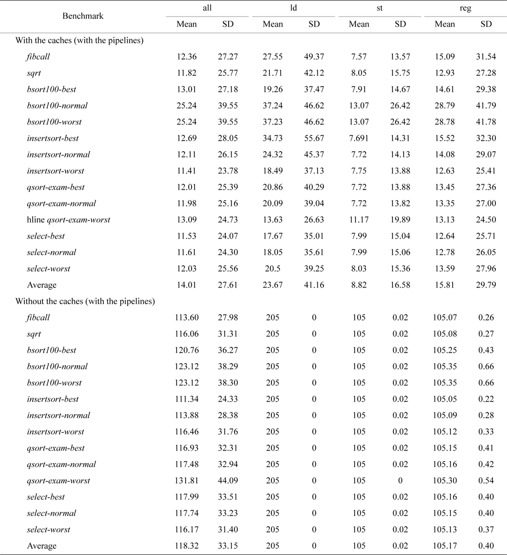
Our second experiment uses the standard deviation of CPI to quantitatively study the effects of caches on the architectural time-predictability of the processors with pipelines, and the results are given in Table 3. As mentioned above, we classify the CPI for different types of instructions, including loads, stores, and other regular instructions. “All” in Table 3 basically represents all the instructions, regardless of their types. As we can see in Table 3, the averaged standard deviation of CPI for load instructions, store instructions, and other regular instructions are 41.16, 16.58, and 29.79, respectively, with caches, while it decreases to 0, 0.02, and 0.4, respectively without caches. This quantitatively demonstrates the time unpredictability caused by cache memories due to the latencies of memory accesses depending on whether or not there is a hit in the caches and which cache is hit. By disabling all caches, the load instructions become perfectly predictable (i.e., the standard deviation of CPI is 0), as there is neither a cache hit nor miss. The store instructions and other regular instructions also become much more time-predictable without caches. However, their standard deviation of CPI is not exactly 0. This is due to the time variation caused by the pipelines, including delays due to control and data hazards as well as various queuing delays. For example, an instruction may need to stay in the instruction window for longer time because it has to wait for the preceding instruction to commit.

It should be noted that the standard deviation of CPI of all instructions does not reveal architectural time-predictability accurately as mentioned earlier. As can be seen in Table 3, the averaged standard deviation of CPI of all instructions with caches is actually smaller than that without caches. This is because the majority of memory accesses with caches result in cache hits, making the latencies of most loads/stores close to those of other regular instructions. This leads to lower standard deviations when compared to that without caches, in which case the loads/stores are guaranteed to miss and thus have longer latencies than other regular instructions, resulting in a higher standard deviation.

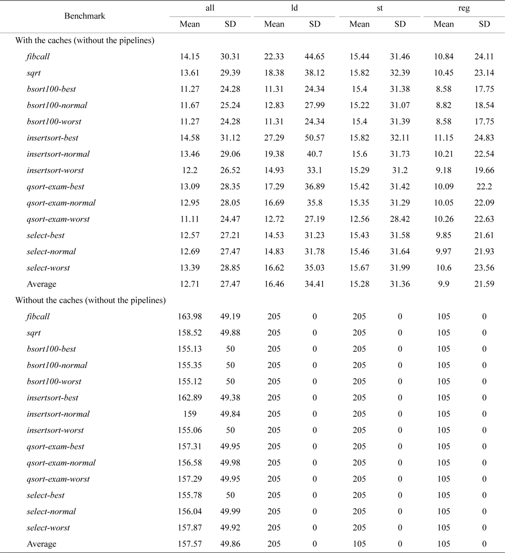
Table 4 compares the mean and the standard deviation of CPI for non-pipelined processors with and without caches. A similar trend can be observed where disabling caches leads to better time-predictability. Moreover, we observe that the standard deviations of CPI of both stores and other regular instructions become 0 without pipelines, indicating that disabling pipelines can further improve time-predictability.

Although both caches and pipelines are detrimental to time-predictability, due to the quantitative nature of our evaluation, we observe that caches can compromise the architectural time-predictability much more than pipelines. This is due to a higher variation of the standard deviation of CPI for each type of instructions between the architectures with caches and without caches when compared to that between the architectures with pipelines and without pipelines (Tables 3 and 4). This may also quantitatively explain why the timing analysis of caches is generally more complex and harder to perform than that of pipelines [1].

[Table 3.] The mean and standard deviation of cycles per instruction for all benchmarks on architectures with the pipelines, with and without caches

The mean and standard deviation of cycles per instruction for all benchmarks on architectures with the pipelines, with and without caches

[Table 4.] The mean and standard deviation of cycles per instruction for all benchmarks on architectures without the pipelines, with and without caches

The mean and standard deviation of cycles per instruction for all benchmarks on architectures without the pipelines, with and without caches

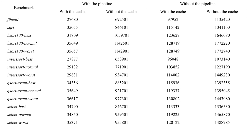
Although architectural time-predictability is degraded by using caches and pipelines, the average-case performance improves with the use of both. As shown in Table 5, the performance of all the benchmarks is best on the architecture with both caches and pipelines and is worst on the architecture without both caches and pipelines. The former is high-performance but not time-predictable, whereas the latter is time-predictable but not high-performance. Among these four architectures, the one with pipelines but without caches seems to provide high time-predictability with adequate performance, better than that without both caches and pipelines. By comparison, the architecture with caches but without pipelines can generally provide good performance, but time-predictability is inadequate. Moreover, architectural innovations are needed to keep high-performance features that do not affect time-predictability and to design new features that are time-predictable and can also boost performance.

[Table 5.] The total execution cycles of all the benchmarks on all the four architectures studied

The total execution cycles of all the benchmarks on all the four architectures studied

Recently, the real-time and embedded computing community has shown interest in defining a metric of time-predictability due to the importance of studying time-predictability quantitatively. Thiele and Wilhelm [2] defined time-predictability as a pessimistic WCET analysis and best-case execution time (BCET) analysis, and Grund [12] defined time-predictability as the relation between BCET and WCET and argued that it should be an inherent system property. Grund et al. [13] then proposed a template for predictability definitions and refined the definition into state-induced time-predictability (SIP) and input-induced time-predictability. Kirner and Puschner [14] formalized a universal definition of time-predictability by combining WCET analyzeability and stability of the system. However, in all the above work, except for that of Grund [12] and Grund et al. [13], the calculation for time-predictability is still dependent on the computation of WCET. Since WCET estimation is usually pessimistic and there is no standard way to compute it (though different methods to derive WCET, such as abstract interpretation and static cache simulation do exist), any time-predictability metric relying on WCET analysis is likely to be inaccurate and would be difficult to be standardized in practice.

Moreover, in all the above work, except again for that of Grund [12] and Grund et al. [13], the definition for time-predictability does not separate the time variation caused by software and hardware, making it overly complicated to derive a time-predictable metric that can effectively guide the architectural design. While Grund [12] and Grund et al. [13] proposed SIP to separate the timing uncertainty between hardware and software, the metric they proposed to evaluate SIP needs to exhaustively find the maximum and minimum execution time of all different states, and this may not be computationally feasible. Also, no quantitative results are given in their study. In contrast, this paper proposes a metric to efficiently assess architectural time-predictability with a quantitative evaluation of architectural time-predictability on statically-scheduled processors with different architectural features.

Recently, Ding and Zhang [15] proposed to use a quantitative architectural time-predictability factor (ATF). Compared to ATF, which can only quantitatively show the ATP of the whole processor, the standard deviation of CPI can provide the ATP for various microarchitectural components, such as caches and pipelines. Thus, we can quantitatively understand the impact of different microarchitectural components on ATP by using the standard deviation of CPI for different types of instructions, a feature which is not available in ATF. Therefore, the standard deviation of CPI can provide useful insights for engineers to design and implement new architectures with better time-predictability.

In this paper, we present the concept of architectural time-predictability to separate that of hardware design from that of software design. We then propose a new metric to evaluate the architectural time-predictability that uses the standard deviation of the clock CPI. Our preliminary evaluation demonstrates that the proposed metric can quantitatively measure time-predictability of processors with different architectural features, such as caches and pipelines.

The standard deviation of CPI can be used to quantitatively guide the design of time-predictable processors. In our future work, we plan to use the standard deviation of CPI to evaluate time-predictability of different architectures, for example branch prediction, multicore designs, etc. Moreover, we intend to use this new metric to quantitatively trade off time-predictability with performance, energy, and cost for real-time systems.