Since the 19th century, ocean wave energy has often been studied as a key renewable energy resource. Over 1000 patented wave energy take-off devices have been proposed as energy converters in the last several decades. Recently, as a specific functional structure system, an array of porous circular cylinders has been studied for use as an efficient wave energy take-off or attenuation system (Park et al., 2010). In general, wave energy take-off techniques are based on nine ideas (McCormick, 2007). One of the most practical and energy efficient concepts is the Oscillating Water Column (OWC), which is based on a pneumatic power take-off inside the chamber achieved by using specially designed air turbines, such as the Wells, Impulse, and Denniss-Auld turbines.
Since Masuda (1971) first proposed a commercially-available OWC device, several commercial-level fixed-type OWC plants have recently been constructed and operated successfully (Heath et al., 2000). Numerical analyses of fixed OWC systems have been performed by many researchers (Brendmo et al., 1996; Wang et al., 2002; Delaure and Lewis, 2003). However, most of these analyses were founded on linear-based numerical models. Koo and Kim (2010) recently developed a fully nonlinear time-domain model of a land-based OWC system. Their simulation included viscous energy loss from the chamber skirt and pneumatic pressure from oscillatory airflows in the chamber.
For a floating-type OWC system, Masuda et al. (1987) proposed a special type of OWC, a Backward Bent Duct Buoy (BBDB), which is thought to be one of the most energy-efficient OWC devices. The BBDB has the typical characteristics of dynamic behavior due to its unique body shape, such as a reverse time-mean drift force. Therefore, many studies on the hydrodynamic behaviors of BBDBs, including reverse drifting, have been conducted, either numerically or experimentally (McCormick and Sheehan, 1992; Hong et al. 2004a; 2004b; Kim et al., 2006; 2007; Nagata et al., 2008; 2009; Imai et al., 2009; Toyota et al., 2008; 2009). Suzuki et al. (2011) performed a numerical investigation to determine the optimal two-dimensional (2D) hull design of the BBDB using the eigen-function expansion method, with the relevant experiment being conducted by Toyota et al. (2010). Using a 2D numerical wave tank (NWT) technique, Koo and Lee (2011) and Koo et al. (2012) calculated the hydrodynamic behavior of a BBDB and chamber free surfaces with different shaped-corners. A proper viscous damping coefficient was applied to their numerical model, which was deducted from the experimental results.
In this study, a state-of-the-art 2D fully-nonlinear NWT technique was fully described for a simulation of a floating OWC wave energy converter, a BBDB. Using the acceleration potential method associated with pneumatic pressured chamber and viscous energy loss, the hydrodynamic performance of the floating BBDB was simulated in the time domain. The developed NWT technique was based on the potential-fluid theory and the boundary element method with constant panels on the boundaries, on which fully nonlinear free-surface and moving body boundary conditions were applied. A mixed Eulerian-Lagrangian (MEL) scheme was used for a time-varying nonlinear free-surface treatment, along with the Runge-Kutta fourth-order time integration scheme, as a time-marching approach. To accurately predict the time derivative of the velocity potential for the freely floating BBDB, the mode decomposition scheme combined with the acceleration potential was implemented to calculate the body force and displacement by simultaneously solving the equations of body motion and the velocity potential.
In order to consider the effect of pneumatic pressure acting on the free-surface inside the chamber, the damped free surface condition was applied to the NWT technique, which was first presented by Evans (1982), Sarmento and Falcao (1985) and Falnes and McIver (1985). A linear relation between the chamber pressure and airflow velocity at the air duct, as observed in various experiments, was used to model the OWC chamber (Gato and Falcao, 1988; Suzuki and Arakawa, 2000). The timevarying pneumatic pressure, due to instantaneous airflow velocity interacting with free-surface fluctuation, was numerically modeled in an OWC system. The energy loss due to viscous flow at the entrance of the BBDB hull, which could be amplified by the body motions, was also modeled by imposing an artificial viscous damping coefficient upon the free surface inside the chamber. In the potential flow calculation, the viscous damping coefficient can be obtained by a comparison of the experimenttal data in open chamber conditions, which represents no pneumatic chamber pressure. The difference of chamber free surface elevation between the potential-fluid-based numerical results and the experimental data in open chamber conditions can be interpreted as the viscous damping.
>
Boundary value problem for a floating BBDB
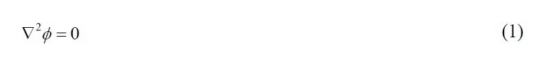
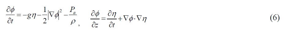
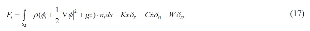
In order to simulate a freely floating BBDB associated with a pneumatic chamber and viscous damping, the mixed boundary value problem has to be solved using proper boundary conditions. The boundaries on the computational domain are the free surfaces inside and outside of the chamber, the body surface, the incident wave boundary, the rigid sea bottom, and the rigid end-wall. Using the velocity potential (
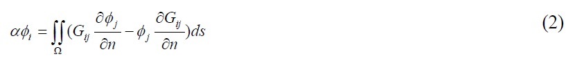
where
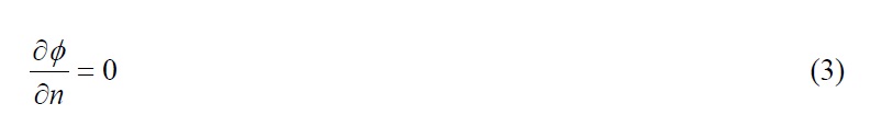
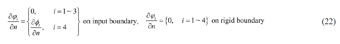
The rigid sea bottom and the vertical end-wall of the computational domain can be described by applying a no-penetration condition so that the water particle velocity in the normal direction is zero on the rigid boundary.
The moving body boundary condition can be expressed by the fact that the water particle velocity adjacent to the body surface is the same as the body velocity in the normal direction:
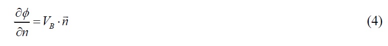
where
where
where
The mixed Eulerian-Lagrangian (MEL) approach was adopted to capture time-varying nonlinear free-surfaces, by which the free-surface boundary conditions can be modified using the total time derivative
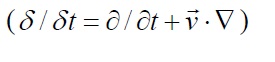
Since the node on the free surface was designed to follow the water particle velocity (
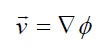
, material-node approach and

is node velocity), the fully nonlinear free-surface boundary conditions were transformed in the Lagrangian frame:
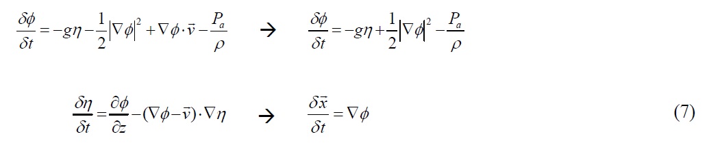
where

is the node location (
During the nonlinear time-domain simulation, nodes on the floating body and the free surfaces must be updated and rearranged using a re-gridding scheme to avoid the numerical instability caused by the local accumulation of material nodes on the surface. The re-gridding process was carried out at every time step for a robust time-domain simulation. An artificial damping zone, as a numerical beach, was placed near the end of the fluid domain to absorb the transmitted waves and to prevent the reflected waves at the end wall. The damping coefficients were applied to both the dynamic and kinematic free surface boundary conditions (Eq. (8)).

where
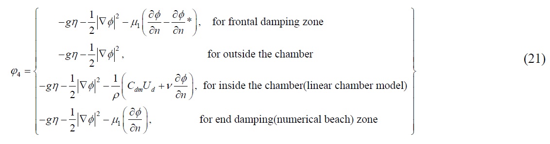
A frontal damping zone was also installed on the free surface in front of the incident wave boundary to prevent a rereflection at the wave maker, which enables long time simulation of surface-piercing bodies. This special damping scheme has to be designed so as to suppress only the reflected waves from the floating body, while preserving the original incident waves. In this regard, the adopted damping term should be applied to the difference between the total waves and incident waves. Then, the free surface boundary conditions can be expressed as:

where
A temporal ramp function at the input boundary was applied during the first two wave periods (2T) to prevent the impulselike behavior of the wave maker and to reduce the corresponding unnecessary transient waves. A Chebyshev five-point smoothing scheme was used along the free surface during the time integration to avoid the non-physical, saw-tooth numerical instability on a highly nonlinear free surface. The smoothing scheme was applied at every fifth time step for a stable time simulation. More detailed explanations of the general numerical schemes and formulations in the NWT technique are given in a previous study (Koo and Kim, 2004).
>
OWC chamber modeling associated with power take-off and viscous damping
The time-varying pneumatic pressure caused by the oscillating water column can be described as the rate of change of air volume inside the chamber (Kim and Iwata, 1991). The rate of air volume change is also directly related to the relative spatialmean vertical velocity between the body and free surface inside the chamber. The pneumatic pressure in the chamber at each time step is expressed as (Koo and Lee, 2011; Koo et al., 2012):
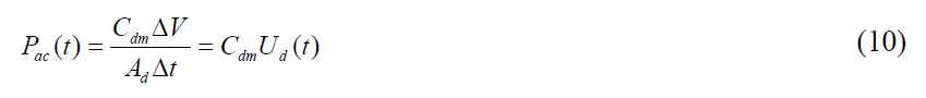
where
In addition to pneumatic pressure, a pressure drop induced by viscous energy loss occurs inside the chamber because a viscous-flow phenomenon, such as vortex shedding, arises at the corner of the BBDB. When the piston-like movement of chamber surface elevation occurs, as in a case of resonance frequencies, and the ensuing high velocity flows are generated, the magnitude of the viscous energy loss greatly increases. In this regard, the difference in the chamber surface elevation between the potential-flow-based numerical solutions and the experimental results can be interpreted as viscous energy loss (work done). A typical entry pressure drop
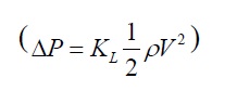
where
Then, the pressure drop in the chamber can be described as (Koo and Kim, 2010):
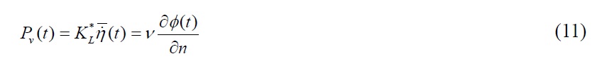
where

denotes a modified energy loss coefficient,

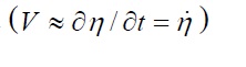
represents the time-varying spatial-mean surface velocity inside the chamber, and
Generally, the pneumatic pressure and viscous energy loss are approximately proportional to the square of the airflow velocity and water column velocity, respectively. Hence, Eqs. (10) and (11), which have an equivalent linear coefficient, can be modified to equations with a quadratic coefficient. The quadratic pneumatic (

where

>
Energy conservation of the BBDB system
The BBDB system contains five energy-flux components: input, reflection, transmission, energy extraction by airflow, and energy loss by viscosity. The transferred wave energy flux into the energy converter is proportional to the square of the wave height and the wave group velocity. Outside the chamber, the energy-flux components per unit area are expressed as:

where

where

>
Acceleration potential method for a freely floating BBDB
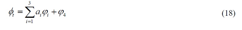
The time derivative of the velocity potential
where

is the horizontal body velocity,
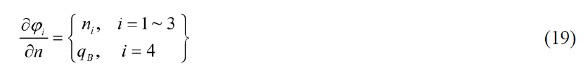
In order to implement the acceleration potential method, we used the mode decomposition method introduced by Vinje and Brevig (1981) to obtain the time derivative of the velocity potential directly from the acceleration field. In a 2D problem, the acceleration field can be decomposed into four modes, corresponding to three unit accelerations for surge-heave-pitch and the acceleration due to the velocity field. Hence, each mode can be obtained by solving the respective boundary integral equation in the acceleration field. Using these four modes and the equation of body motion, the body acceleration can be determined.
The time derivative of the velocity potential
where
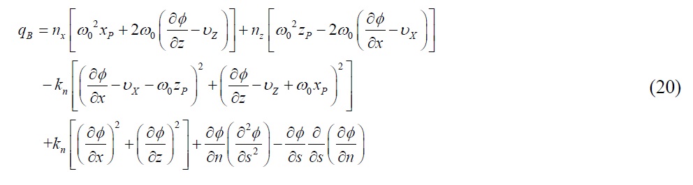
To solve the boundary integral equation for each mode in the acceleration field, the body boundary condition is given as:
where,
where
The free-surface boundary conditions for the respective free surface areas of the BBDB system in the acceleration field are also given as:
where
After solving the boundary integral equation in the acceleration field for the aforementioned conditions,


where
,
From Eqs. (23) to (25), three unknown accelerations (
In the present study, a freely floating BBDB with no additional mooring lines was used to evaluate the hydrodynamic performance. Therefore, neither horizontal spring nor damping coefficients was applied to Eq. (23). In the fully nonlinear simulation, the instantaneous position of the BBDB was updated at every time step and the body drifts during the time simulation.
In order to verify the calculated results from the developed numerical model, an experiment was conducted independently in the 2D wave tank at the University of Ulsan (Koo and Lee, 2011). The wave tank dimensions were 0.5 × 0.4 × 35
Table 1 shows the specifications of the BBDB model used in Koo and Lee (2011). Since the width of BBDB model is 0.48 m compared with the tank width (0.5
Since the wave maker used in the present experiment cannot control the reflected waves from the floating body, the re-reflection may occur when the duration of wave generation is long. Therefore, the steady-state waves with no contamination from the re-reflected waves are only used to compare the numerical results.
[Table 1] Specifications of the BBDB model.
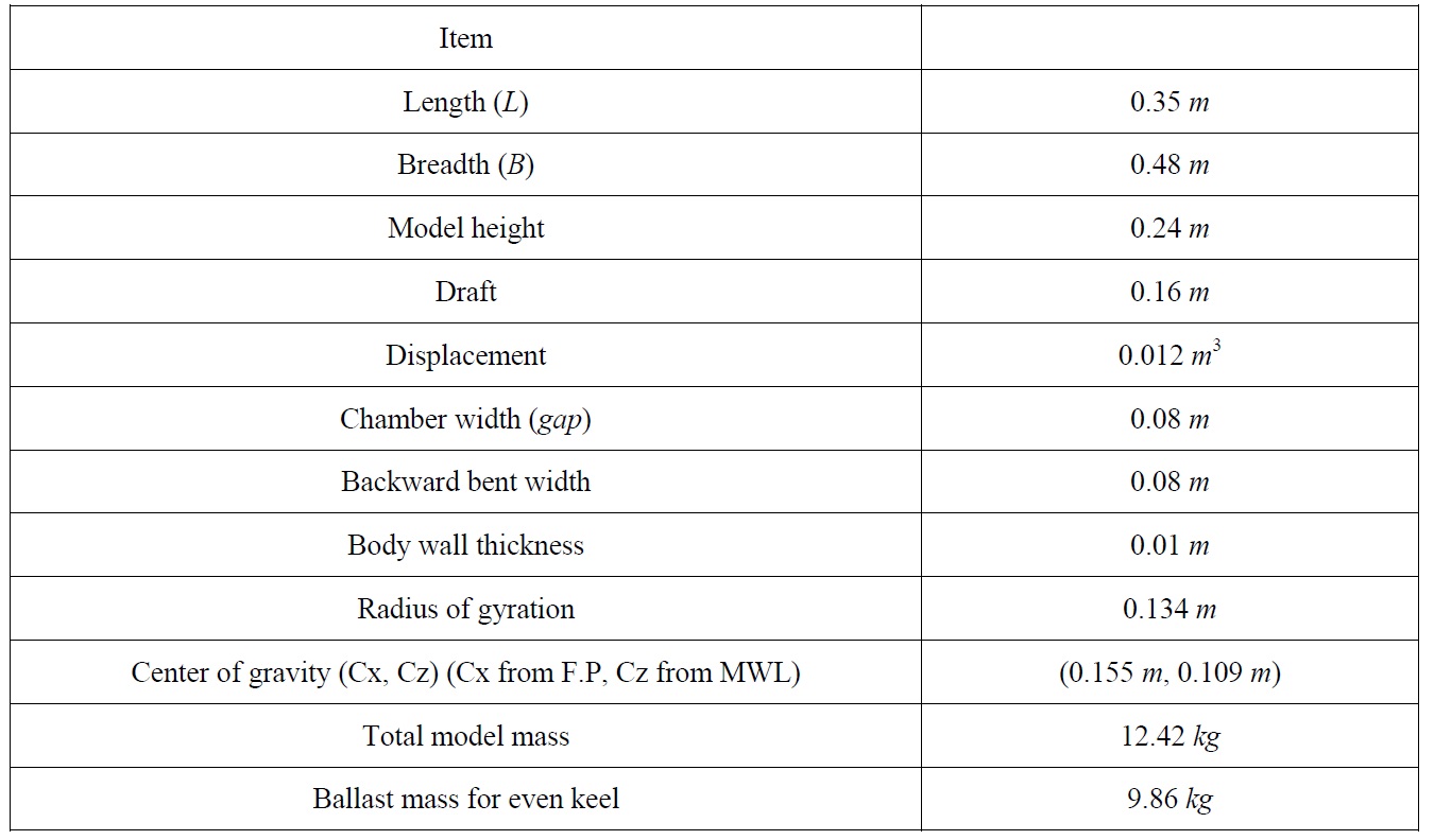
Specifications of the BBDB model.
NUMERICAL RESULTS AND DISCUSSION
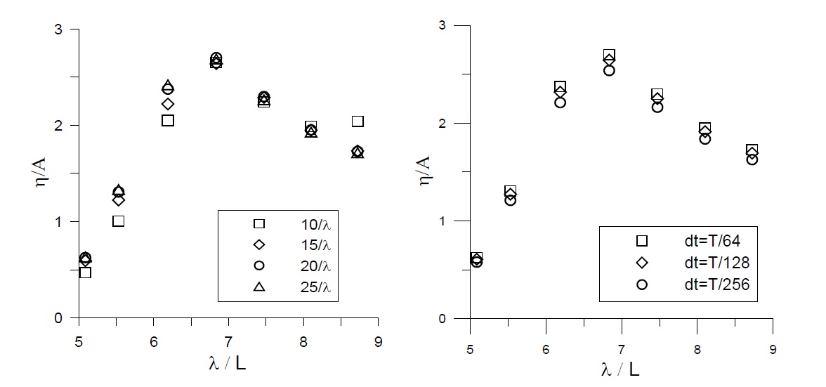
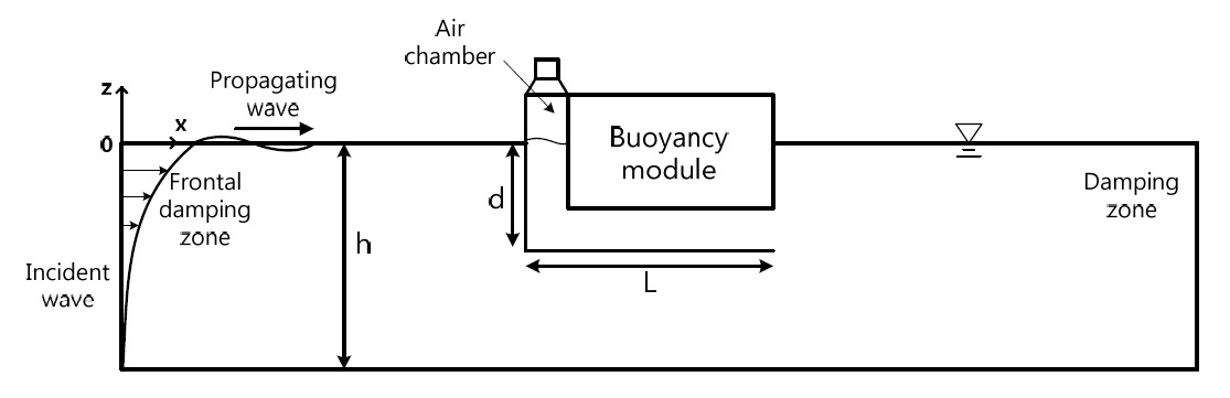
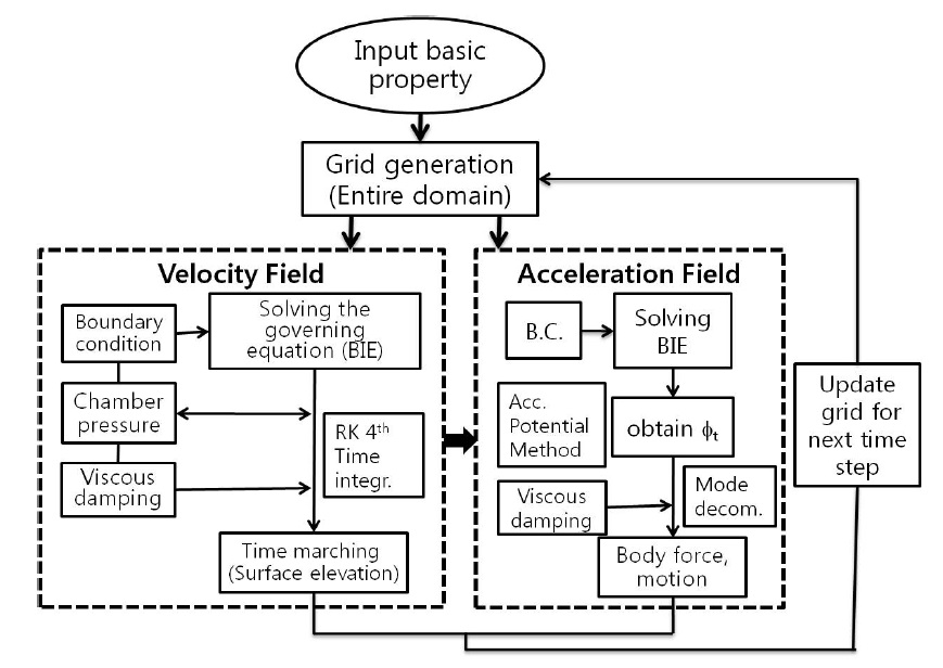
A schematic diagram and coordinate system for the present numerical model is shown in Fig. 1. The flowchart of computational algorithm is also shown in Fig. 2. The dimensions of the BBDD are the same as those in the experimental model (Table 1). Each side of the free surface (weather and lee side) is four times the incident wavelength ( 4
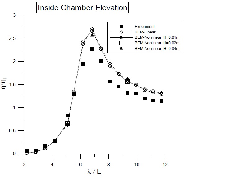
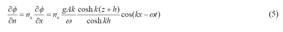
Initially, the calculated wave elevations of the fixed BBDB were compared with the experimental data (Fig. 4) to determine the viscous energy loss due to the body shape. The linear and nonlinear results were also compared to evaluate the effect of nonlinear interactions between wave and body. A significant difference was observed between the numerical and experimental results near the resonance frequencies, where the incident wavelength was approximately six times greater than the total body length (
Since a small incident wave steepness was applied to the entire frequency range ( 0.00243 <
The discrepancy between the numerical and experimental results in the resonance frequency was caused by viscous loss. Energy loss due to vortex generation may occur at the sharp corners of the BBDB.
In order to compensate for the viscous energy loss with the artificial damping in the fixed BBDB system, a small viscous damping coefficient (
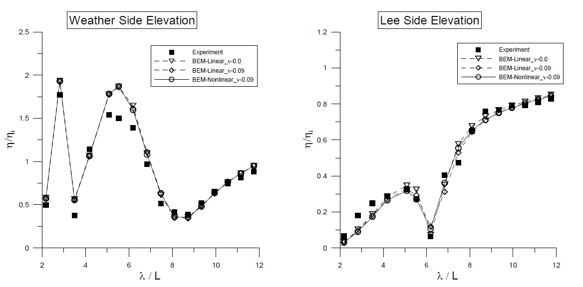
A comparison of surface elevations at the weather and lee sides is shown in Fig. 6. All data were measured at 1
results. It is also observed that a slight difference between the cases of viscous damping and no damping, which implies that the effect of a small viscous damping coefficient (
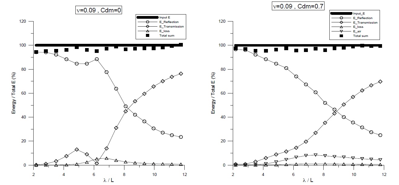
Total energy conservation of the fixed BBDB system is compared in Fig. 7. For the open chamber conditions (
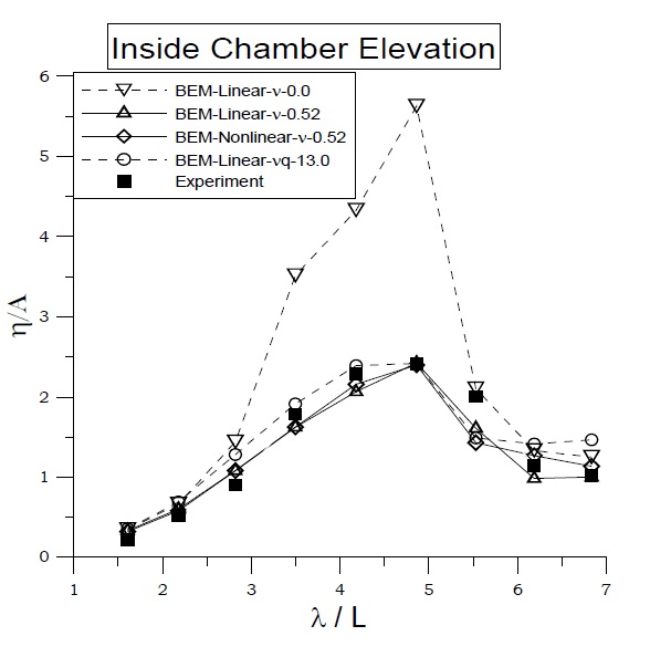
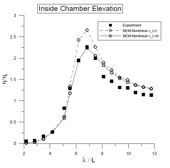
For the floating BBDB system, Fig. 8 shows the comparison of chamber surface elevations for the experimental and numerical calculations. With a tuned linear equivalent viscous damping coefficient (
The proper viscous damping can be obtained from a comparison of the experimental data with the open chamber conditions, where the viscous energy loss only exists without pneumatic pressure. The viscous damping coefficients shown in the figures were divided by water density ((
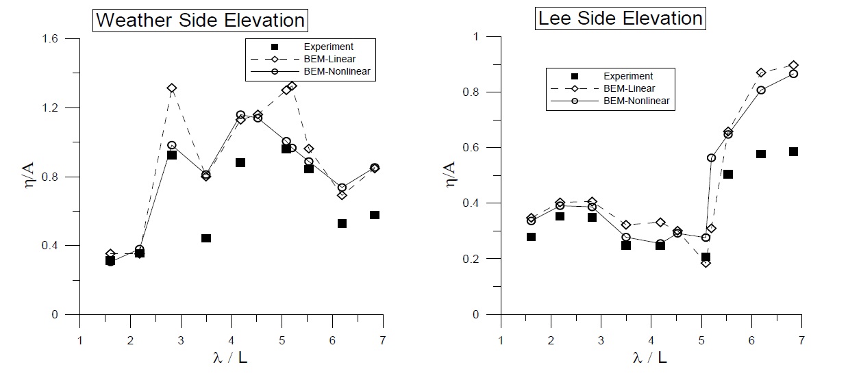
Fig. 9 shows a comparison of the surface elevations at the weather and lee sides of the BBDB with the application of a linear viscous damping coefficient inside the chamber free surface. The calculated elevations agree reasonably well with those from the experimental data. Due to the difficulty in controlling the reflected waves in the floating body experiment, the measured elevations deviate from the numerical results at some frequencies, especially in the long wave region. Since a relatively large motion of the BBDB magnifies the radiated waves, the nonlinear calculation results with updated body and free-surface motions showed greater accuracy than the linear results calculated with a mean-positioned body and free surface. The magnitude of elevation at the lee side is smaller near the resonance frequency region (
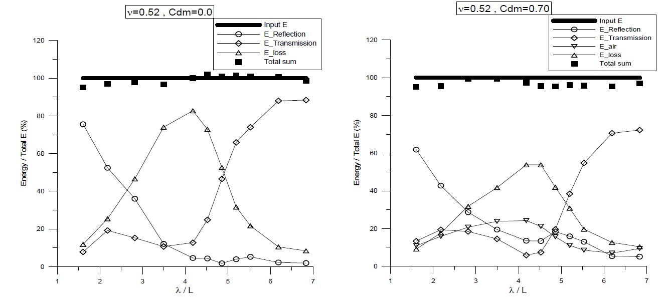
The respective energy components of the floating BBDB for both chamber conditions are compared in Fig. 10. In the open chamber conditions (left graph), as pointed out by Koo and Lee (2011), the relative energy loss by viscosity near the resonance frequencies is up to 80% of the incident wave energy, which indicates that a large amount of energy could be lost at the sharp corners of the body by the resonant pitch-induced vortices. In the pneumatic chamber conditions (right graph), the relative energy loss can be reduced by 50% of the total energy. This can be explained by the fact that the motion of the BBDB decreesed due to the effect of the pneumatic pressured chamber, resulting in a diminished vortex generation. In both chamber conditions, the total energy in the computational domain was conserved over the whole range of frequencies. Comparing with Fig. 7, the magnitude of the pneumatic energy in the floating case (about 25% of incident energy) was greater than that in the fixed case (about 10%). Thus, the body motion (heave and pitch) may amplify the relative vertical water column velocity, thus increasing the resultant airflow velocity.
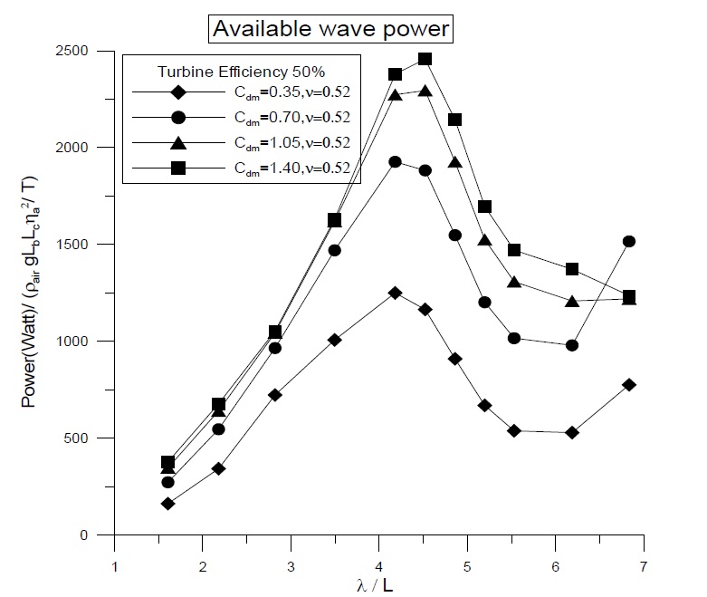
A comparison of the available wave power with various pneumatic coefficients (
The hydrodynamic performance of a floating OWC device was evaluated in the time domain. An acceleration potential method using full-updated matrix calculation, associated with a mode decomposition scheme, was implemented to obtain the hydrodynamic force and displacement of a freely floating BBDB. The developed NWT technique was based on the potential theory and the boundary element method with constant panels on the boundaries, on which fully nonlinear free-surface and moving- body boundary conditions associated with OWC power take-off were applied. The modeling of the pneumatic chamber and viscous damping was proportional to the square of the airflow velocity and water column velocity, respectively. However, the numerical model can also be simplified to a linear relation. Open sea conditions can be realized in the computational domain by using the frontal damping and the numerical beach. Therefore, the NWT technique was better than the experiment in controlling the reflected waves from the wave maker and floating body.
A significant difference of chamber surface elevation was observed between the numerical and experimental results near the resonance frequencies, which may be attributed to the viscous energy loss. The energy loss by vortex generation may increase at the sharp corners of the BBDB. The numerical results under the open chamber conditions were adjusted by adding a proper viscous damping coefficient, obtained from a comparison of the experimental data. The calculated surface elevations affected by pneumatic pressure correlated reasonably well with the experimental values.
The total energy summation of the BBDB system in the computational domain was found to be conserved over the whole range of frequencies. In the case of a floating BBDB with an open chamber, the relative energy loss due to viscosity near the resonance frequencies was up to 80% of the incident wave energy, which indicates that a large amount of energy could be lost at the sharp corners of the body by the resonant pitch-induced vortices.
Since a relatively large motion of the BBDB magnified the radiated waves, the nonlinear results that were calculated using the updated free-surface and body motions were found to be more accurate than the linear ones with a mean-positioned free surface and body.
The developed NWT model for a floating BBDB device can be used to analyze the hydrodynamic performance of a floating-type OWC system. Using a parametric study for various conditions compared with the corresponding experiments, it is possible to predict the motion characteristics and determine the proper BBDB shape for various environmental conditions.