Simulations of cavitation flow and hull pressure fluctuation for a marine propeller operating behind a hull using the unsteady Reynolds-Averaged Navier-Stokes equations (RANS) are presented. A full hull body submerged under the free surface is modeled in the computational domain to simulate directly the wake field of the ship at the propeller plane. Simulations are performed in design and ballast draught conditions to study the effect of cavitation number. And two propellers with slightly different geometry are simulated to validate the detectability of the numerical simulation. All simulations are performed using a commercial CFD software FLUENT. Cavitation patterns of the simulations show good agreement with the experimental results carried out in Samsung CAvitation Tunnel (SCAT). The simulation results for the hull pressure fluctuation induced by a propeller are also compared with the experimental results showing good agreement in the tendency and amplitude, especially, for the first blade frequency.
The practical importance of accurate numerical simulations to predict the cavitation pattern and hull pressure amplitude has increased in the field of ship building industries. The researches to simulate the cavitation flow using RANS solver were performed actively in the last several years because cavitation models for RANS solver and computation power have been rapidly developed in the last decade.
Watanabe et al. (2003) performed a pioneering study on the cavitation flow for a marine propeller using RANS. Salvatore et al. (2009) compared seven computational models using RANS, LES, and BEM for the INSEAN E779A propeller in the uniform flow and the wake field. The cavitation simulation for conventional and highly-skewed propellers in the behind-hull condition using an in-house RANS solver was performed by Shin et al. (2011). Hasuike et al. (2010) simulated the cavitation flow and showed a possibility to predict the cavitation erosion risk with the indexes using time differential of cavity void fraction or pressure.
On the other hand, the usage of commercial CFD software gradually increased to simulate the cavitation flow for marine propellers. Boorsma and Whitworth (2011) used STAR-CCM+ to study on the prediction of cavitation and erosion for a propeller and rudder. Bertetta et al. (2011) compared the results of RANS solver using STAR-CCM+ with those of potential solver for the cavitation flow of a controllable pitch propeller. Morgut and Nobile (2011) studied on the performance of three cavitation models for a marine propeller using ANSYS-CFX. Li and Terwisga (2011) used FLUENT to investigate unsteady cavitation phenomena for 2D and 3D foils. Kawamura (2010) assessed cavitation erosion risk based on pressure impacts and simulated the cavitation flow and the amplitude of pressure fluctuation for a marine propeller using FLUENT.
Most of simulations except for Kawamura (2010) prescribed a velocity distribution at the inlet boundary of the computational domain to achieve the wake field at the propeller plane. In that case, the adjustment of inlet boundary condition to get a desired velocity contour at propeller plane is of primary importance and very laborious work. Therefore, Kawamura (2010) used a full hull body to generate the wake field at propeller plane. Nevertheless, the cavity extent was under-predicted and the pressure amplitudes were about 70% of the experimental results.
In this paper the results of numerical simulations using RANS for the cavitation pattern and hull pressure fluctuation of marine propellers are presented. A commercial CFD software FLUENT version 14.0 is used for the numerical simulations. The cavitation model of Schneer and Sauer (2001) is applied to simulate the cavitation flow. A computational domain including a full hull body submerged under the free surface is used to simulate directly the wake field at the propeller plane. Two kinds of studies varying cavitation number and propeller geometry are executed in order to validate the numerical simulation method. And the numerical simulations are performed at the same as the test conditions in the cavitation tunnel and compared with the experimental results.
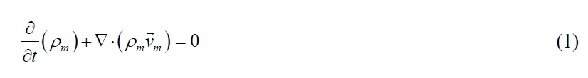
A commercial CFD software FLUENT version 14.0 was used for the numerical simulations, in which the cavitation flow was solved by a mixture model based on a single-fluid multiphase mixture flow approach.
In the mixture model, the continuity equation and the momentum equation become as
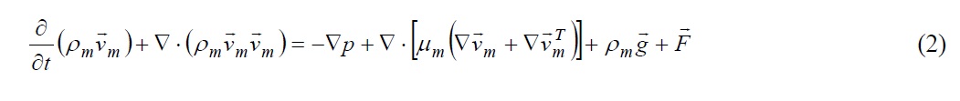
The mixture density and viscosity coefficient are defined as
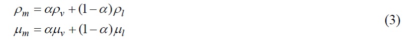
where
The cavitation model of Schneer and Sauer (2001) applied in this research solves the vapor volume fraction with following transport equation:
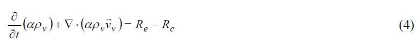
where the terms in the right hand side,
when
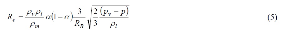
when
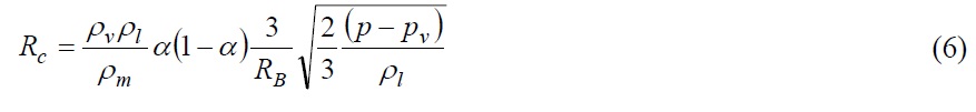
Here, the bubble radius,
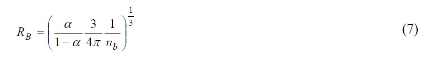
where
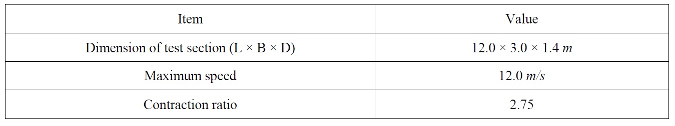
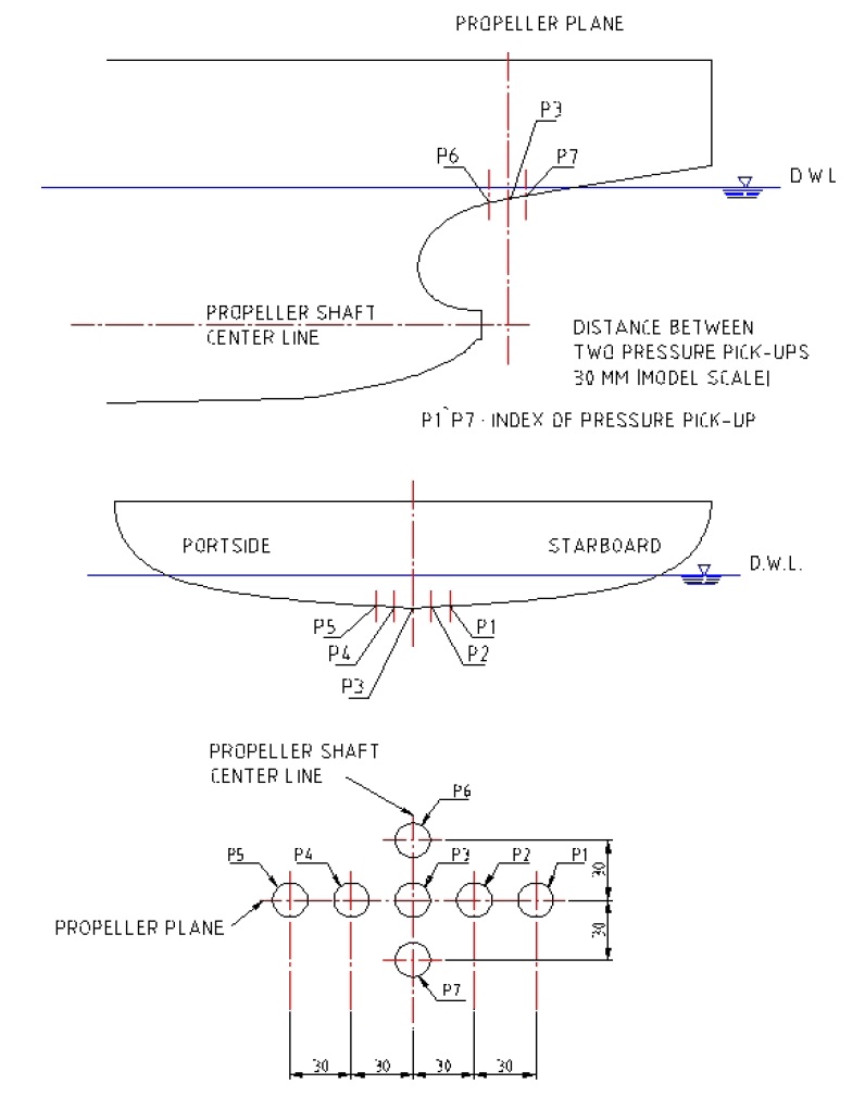
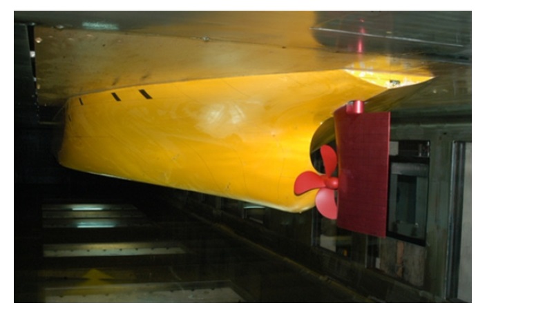
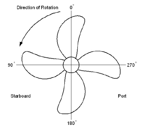
Model tests to observe cavitation flow on a propeller blade and to measure pressure fluctuation on a hull surface induced by the propeller cavitation were carried out in Samsung CAvitation Tunnel (SCAT). The principal particulars of the test section of SCAT are summarized in Table 1 and the set-up of a model ship and propeller is shown in Fig. 1. The definition of propeller blade angle is depicted in Fig. 2. The propeller blade angle begins from the top position toward propeller rotation direction. Pressure transducers to measure the pressure fluctuation on a hull surface were installed on the top of propeller with the intervals of 30
[Table 1] Principal particulars of the test section of SCAT.

Principal particulars of the test section of SCAT.
The length of the model ship, a crude oil tanker, was about 7.6
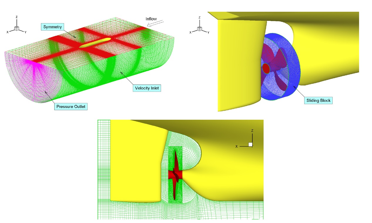
To simulate the propeller cavitation flow under similar situation to the model test, a full hull body submerged under the free surface was modeled in the computational domain. The free surface was substituted with a symmetry boundary condition because the mixture model for the cavitation flow and the Volume of Fluid (VOF) model for the free surface could not be implemented simultaneously in FLUENT.
A sliding block surrounding the propeller, composed of unstructured girds, was applied to implement the effect of propeller rotation. Pyramid cells were used for the surface of propeller and boundaries, and tetrahedral cells were filled in the block. On the other hand, structured girds were applied to the other domains expect for the sliding block. Fig. 4 shows the outline of grid system including boundary conditions and the interface between sliding and other blocks. While the test section of the cavitation tunnel was rectangular, a half circular sectional profile was used for the computational domain to achieve a good grid quality of structured grid. The grid sizes were 1.4
As the numerical model for cavitation flow, Schneer and Sauer (2001) was applied in this research. Bubble number density was set as 1e+15, which corresponds to the bubble radius of 3
A propeller coated with the rough paint tended to increase the cavity extent and pressure fluctuation as compared with a smooth surface propeller in the experiment. However, since it was impossible that the effect of the paint was implemented in numerical simulation, a smaller cavitation number was used for the simulation instead of the rough paint. The adjustment was approached with ignoring a wave height at stern which was considered in the model test.
[Table 2] Summary of simulation methods.
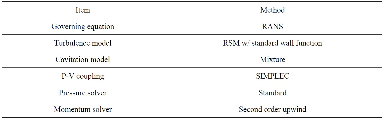
Summary of simulation methods.
In this research two kinds of simulations were executed and compared with the experimental results. The first simulation was performed at two draught conditions to investigate the effect of cavitation number. The other study was to validate the detectability of the numerical simulation about the differences of cavitation pattern and pressure amplitude from the small modification of propeller geometry.
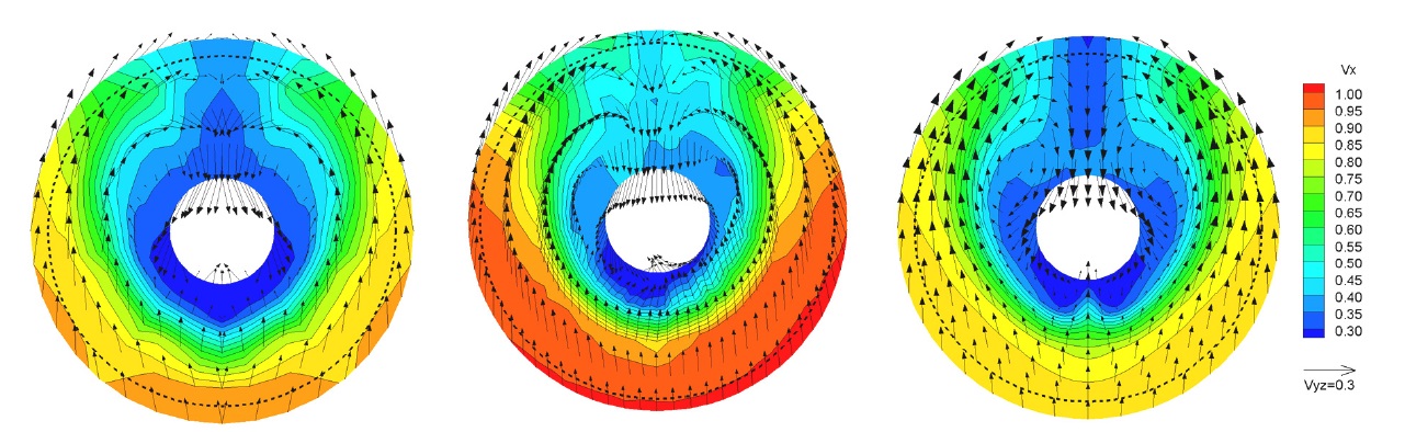
Prior to the cavitation simulation, the bare hull without the propeller was simulated to compare the wake field at the propeller plane. Fig. 5 shows the comparison of velocity contours and vectors between the experimental data and simulation result at the propeller plane. Model ship speed was 1.35
The simulations were performed at design and ballast draught conditions, and the simulation results were compared with the experimental results of SCAT. The propeller tested in the model test is a 4-blade propeller (Prop-A) designed for a crude oil tanker. Mean pitch ratio and expanded area ratio of the propeller are 0.655 and 0.480, respectively. The simulation conditions are summarized in Table 3. The cavitation number is defined as
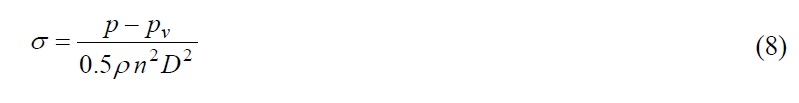
where
[Table 3] Summary of simulation conditions to study the effect of draught condition.
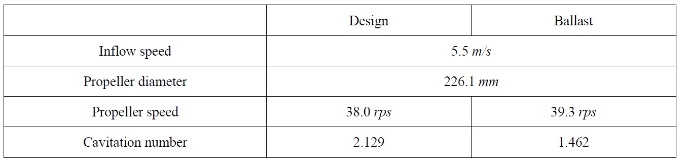
Summary of simulation conditions to study the effect of draught condition.
The thrusts of the simulations at the design and ballast conditions were about 4% higher than those of the experiments. The larger thrusts of the simulations result from the slower axial velocity at the propeller plane as compared in Fig. 5.
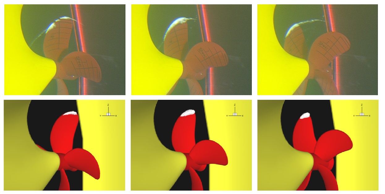
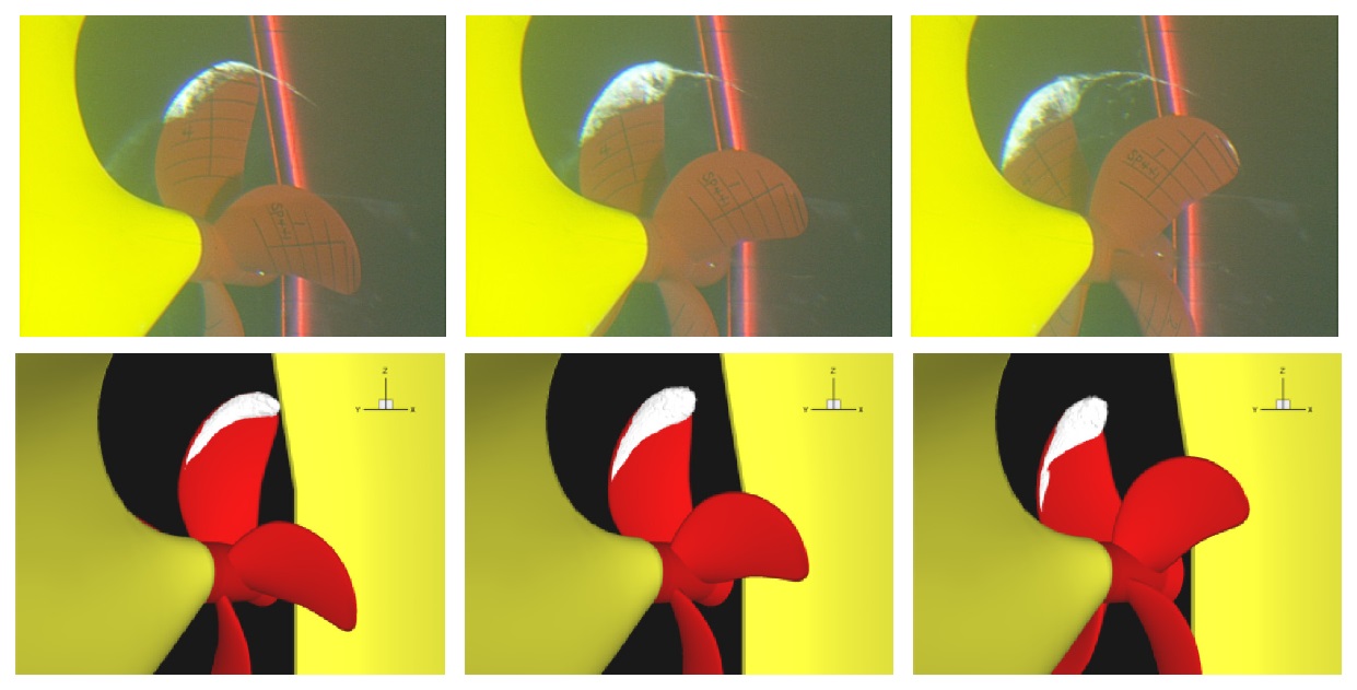
Cavitation patterns at the propeller blade angle of 0°, 20°, and 40° at the design and ballast draught conditions are compared with the experimental results in Figs. 6 and 7. The cavity extent in the simulation are expressed with the isosurface of
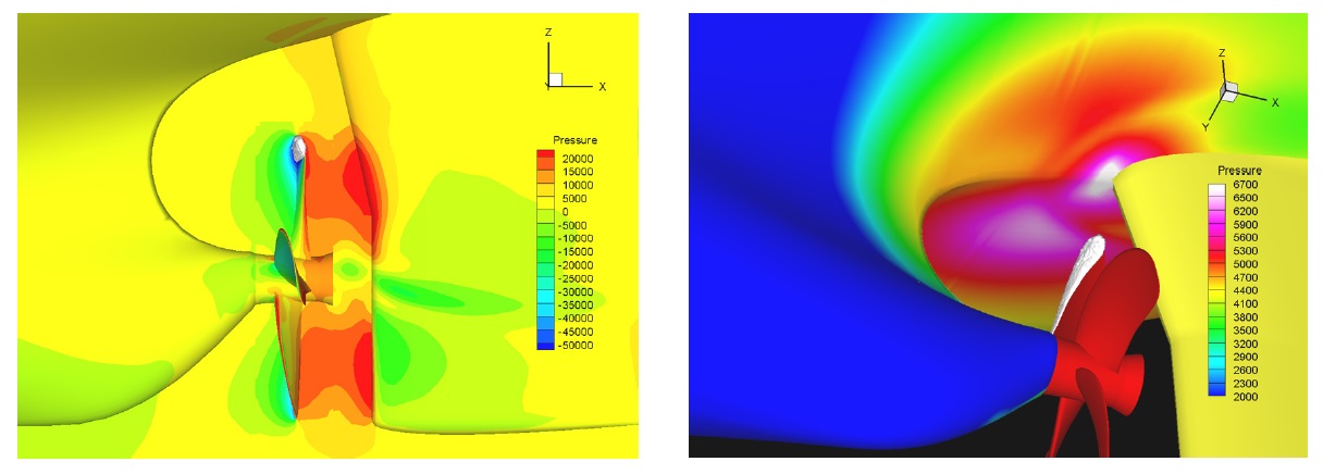
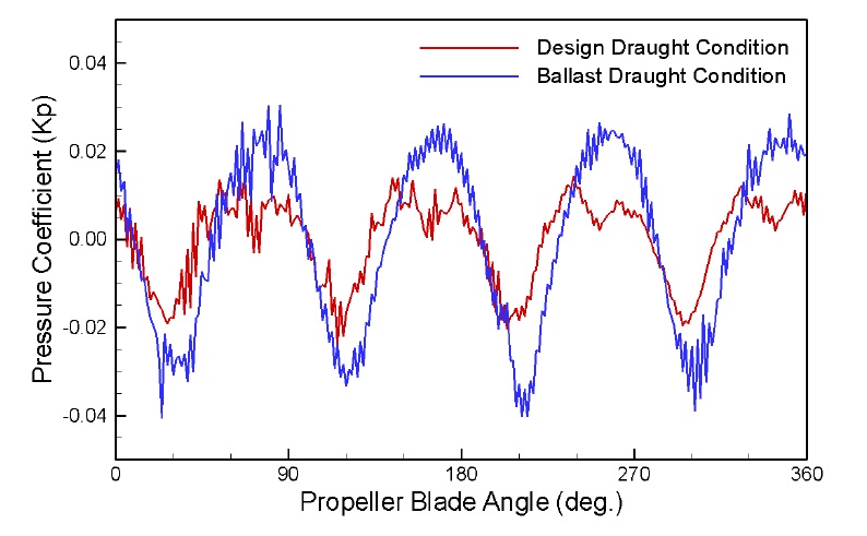
Fig. 8 shows an instantaneous pressure distribution on the hull surface induced by the propeller cavitation as well as field velocity around propeller in x-z plane section. Very high pressure concentrates above the propeller position, especially on starboard side rather than port side. Time histories of pressure fluctuation on P2 transducer at the design and ballast draught conditions are plotted in Fig. 9. Hull pressure is expressed with the pressure coefficient defined as
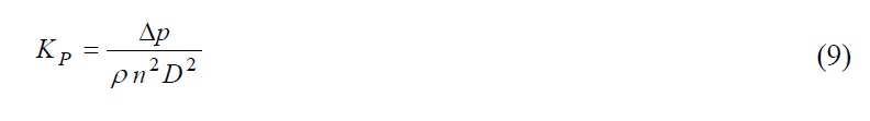
where Δ
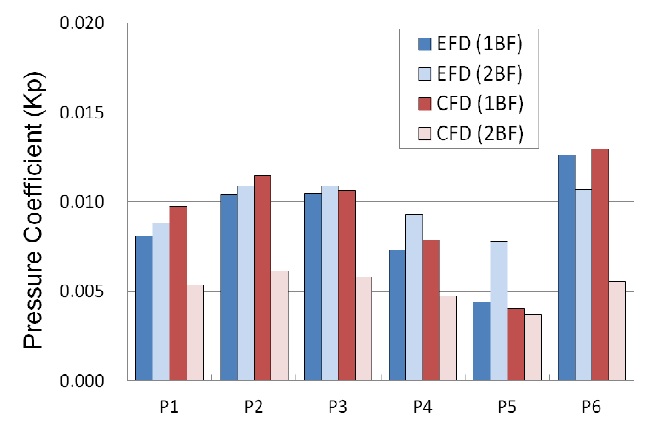
The hull pressure amplitudes for Prop-A at the design draught condition are compared with the experimental results in Fig. 10. Since the position of P7 was concealed beneath the rudder trunk, P7 could not be measured in this research. For the first blade frequency (1BF), the simulation results show good agreement with the experimental results in the tendency and magnitude of pressure fluctuation, but the pressure amplitudes of P1 and P2 at starboard side are about 20% and 10% higher than the experiments, respectively. At the other pressure transducers, the pressure amplitudes are very similar to the experiments. The second blade frequencies (2BF) of the simulation are almost half of the experimental results, even though the tendency is similar to the experiments. As explained in Fig. 5, the gradient of axial velocity around 20° and 340° probably affects the increase of 2BF amplitude in the experiment. In contrast, the velocity gradient in the simulation is very smooth, resulting in relatively small amplitude of 2BF. And the numerical diffusion and grid fineness around the propeller tip might be another reason for smaller 2BF amplitude in the simulation. Overall, the hull pressure amplitudes of starboard side are higher than port side, and the pressure amplitude of P6 located upstream from the propeller plane is higher than P3 located at the propeller plane.
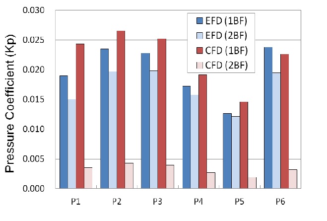
Fig. 11 shows the comparison of the hull pressure amplitudes at the ballast draught condition with the experimental results. The amplitudes of 1BF are about 10% higher than the experiments except for P1 and P6. The pressure amplitude of P1 is about 28% higher than the experiment, while that of P6 is about 5% lower. Nevertheless, the tendency of pressure amplitude is very close to the experiment. However, the amplitudes of 2BF are significantly lower than the experiments because the effect of axial velocity gradient in the simulation may be diminished due to the relatively large cavity extent in the ballast draught condition. This phenomenon can be explained through Fig. 9. The two peaks with the interval of about 40° at the crest of the signal observed in the design load condition are not observed in the ballast condition.
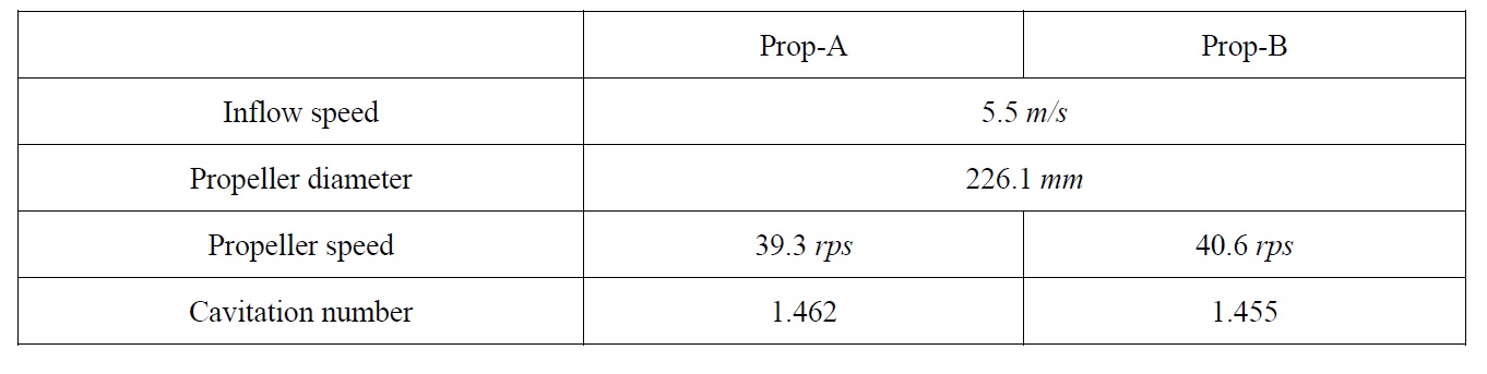
Another propeller (Prop-B) was designed to study on the effect of propeller rake distribution. Prop-B has the backward rake of 0.014D at tip, while Prop-A has the forward rake of 0.007D at tip. The other parameters for propeller geometry such as pitch, camber, and chord including propeller diameter are exactly same. Due to the rake distribution, the rotation speed of Prop-B is slightly higher than that of Prop-A; as a result, the cavitation number of Prop-B is relatively lower than that of Prop-A. The simulation conditions for Prop-A and Prop-B are summarized in Table 4.
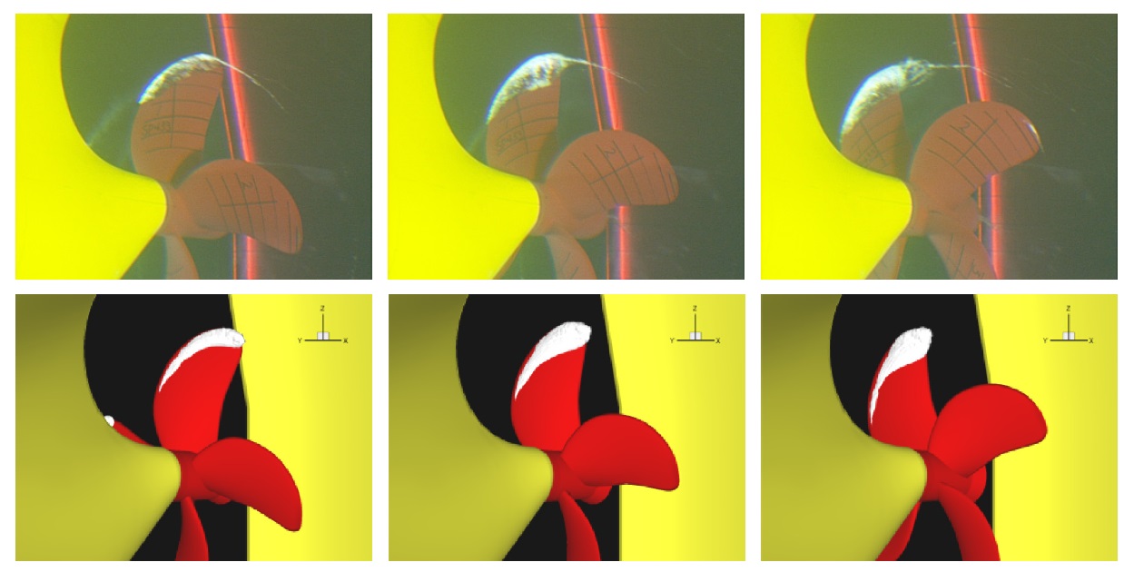
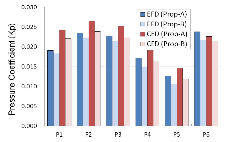
The cavitation patterns at the ballast draught condition for Prop-B are compared with the experimental results in Fig. 12. The cavity extents of Prop-B are not different from Prop-A in both experiment and simulation. However, the effect of propeller rake is distinguished in the hull pressure amplitude as shown in Fig. 13. Prop-B with the backward rake reduces the pressure amplitude of about 5% at P1 to P3 and about 13% at P4 and P5 in the experiment. Similarly, the amounts of reduction are about 10% at P1 to P3, about 5% at P4 and about 10% at P5 in the simulation. From the simulation results, it can be concluded that the numerical simulation using RANS is useful to detect the difference of pressure amplitude due to the small modification of propeller geometry.
[Table 4] Summary of simulation conditions to study the effect of propeller geometry.

Summary of simulation conditions to study the effect of propeller geometry.
Numerical simulation studies using RANS for cavitation flow and hull pressure fluctuation of marine propellers were presented in this paper. A computational domain including a full hull body submerged under the free surface was used to simulate directly the wake field at the propeller plane. And the simulation results were compared with the experimental results performed in the cavitation tunnel.
Two kinds of studies were executed in this research. At first, the numerical simulations were performed in design and ballast draught conditions to study the effect of cavitation number. The cavitation patterns at both conditions agreed well with the experimental results. The first blade frequencies of the pressure fluctuations in the simulations were slightly larger than the experiments, whereas the tendency of the pressure amplitudes according to the location of the transducers was very similar to the experiments. However, for the second blade frequencies the simulations showed some limitations to predict the magnitude of pressure fluctuation due to the difference of wake field at the propeller plane. The other study was to validate the detectability of the numerical simulation for the cavitation pattern and hull pressure amplitude. Two propellers with slightly different geometry were simulated and compared with the experimental results. The cavity extents of the simulation and experiment were not different between two propellers. However, the pressure amplitudes of two propellers had small difference, and that was validated in the numerical simulation.
In conclusion, the cavitation simulation using RANS showed reliable performance to predict the cavitation pattern and hull pressure amplitude through this research. To improve the accuracy of 2BF harmonics in the simulation, however, numerical methods to achieve more accurate wake field at the propeller plane need to be studied in detail. For the further work, various ship types will be simulated and compared with experimental data to evaluate this numerical simulation method.