If pressure in any point of fluid flow is lower than fluid vapor pressure at that temperature, bubbles may be formed in the fluid flow which is named cavitation. Cavitating flows are defined by multi-phase flow regions. The two phases that are the most important are the water and its own vapor. The most cavitation patterns which occur on marine propellers usually comprise one or more of the following types: sheet, bubble, cloud, tip or hub cavitation (Nakamaya, 1998).

Sheet cavitation appears on the propeller near of the blades leading edges. If the inflow resultant velocity enters to the propeller blade in positive angles of attack, sheet cavitation occurs on backside or suction surface, and if it enters in negative angles of attack this cavitation appears on propeller face surface.

Considerable work has been done in attempting to model cavitation numerically. Uhlman (1987) has applied BEM to the 2D hydrofoil, in which the velocity with the re-entrant jet model was used and cavity surface obtained in an iterative solution process till complete satisfaction of dynamic and kinematic boundary condition. During the last two decade, many researchers have been accomplished on the hydrofoils and marine propeller using BEM and Computational fluid dynamics (CFD). Predictions of the propeller performance in unsteady flow by Hsin (1990) and unsteady cavitation investigation flow on the propeller by Fine (1992) are the examples of these researches using BEM. Fine’s work was followed by Kinnas and Fine (1994). In addition, similar works in this area have been done by Kim and Lee (1996).Also, interaction between propeller cavitation and rudder carried out by Lee, et al.(2003), cavitating hydrofoils and marine propeller by Ghassemi (2003), hydroelastic analysis of propeller cavitation by Young (2003), modeling of cavitation caused by blade tip vortex by Lee and Kinas (2002), were performed. Hong (2008) investigated the cavitation on the marine propellers with and without consideration of the viscosity effect. A design method for increasing performance of the marine propellers including the Wide chord tip (WCT) propeller is suggested produces very low fluctuating pressures comparing with conventional propellers (Lee et al., 2010).

In this study, the numerical modify BEM based on potential is used to analyze wetted flow and sheet cavitation on propeller. In this analysis, flow detachment point of minimum pressure point, closest point to detachment point of real flow in comparison with blade leading edge points and smooth point of blade surface, has been considered. Also, potential of detachment point of flow which is a common point between points under cavitations and points of wetted flow has been investigated and modified.

In this article modified minimum pressure point is selected as a detachment point in sheet cavitation analysis. In other words according to solution algorithm in first step the fully wetted flow analysis is executed on marine propeller and in the second step, minimum pressure points will be derived and the initial detachment points will be determined based on the second step.

Then to increase the accuracy and avoid jump in potential values between wetted and cavitating areas, the detachment point potential will be derived based on the three previous potential points in chord direction of the wetted area. On the other hand the detachment point potential value will be calculated from the previous points continuously, considering an extrapolation function of order 2.

In such a way that there will be a continuity between the potential values of wetted and cavatating points. In present study the effect of cross flow on cavity surface determination is applied. As it can be seen, there is a better agreement between the numerical results gained from the present method and fluent results than hung-song method. The error rate near the tip blade is owing to the lack of tip vortex modeling.

In order to increase the accuracy of cavity area, volume fraction, detachment point location, detachment point potential was modified and the cross flow effect is applied, using the present method which will be discussed in during the article.

Based on the assumptions that the fluid in the boundary domain is incompressible, inviscid and irrotational, the body is subjected to the inflow uniform velocity at the upstream of the flow. Then, the perturbation velocity potential over solution field is irrotational except non-continued surfaces of velocity field which constitute lifting surface wake of body. In other word, to use Laplace’s equation for modeling fluid flow around propeller, the flow shall be irrotational in all points of the field except some discontinuity points which propeller wake is replaced by them.

The disturbance velocity, being irrotational, may be written as the gradient of the disturbance potential. For incompressible fluid flow, continuity equation ∇・V=0, converts to Laplace equation as follow.

Total velocity in each point of fluid field Ω , is equal to summation of perturbation velocity and non-perturbation velocity.

For an incompressible, inviscid and irrotational flow the Navier-Stokes momentum equations reduce to the Bernoulli equation. In the body-attached reference system, the steady Bernoulli equation reads:

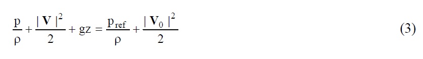
In Eq. (3) p, ρ and p_ref are pressure, fluid density and reference pressure of the fluid, respectively. For a propeller, p_ref is the pressure far upstream and it obeys to the hydrostatic law, p_ref = p_atm ρgz being p_atm the atmospheric pressure at the depth of free surface. Two important dimensionless parameters, pressure coefficient and cavitation number, are defined as follow:

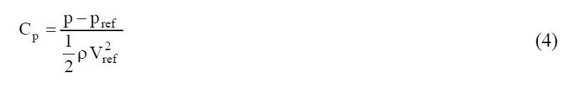
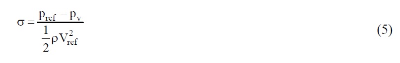
In Esq. (4) and (5), p_v is vapor pressure and V_ref is reference speed. For propellers, reference speed is usually considered as the resultant vector of inlet velocity and rotational speed (nD). D is the propeller diameter and n is the rotational speed (revolution per second). V_ref is defined as:

Dynamic equation (3) can be rewritten as:

In order to solve the Laplace equation in the external flow around propeller, Eq. (1), boundary conditions should be imposed on each of the surfaces that bound the fluid domain. Considering the boundary surface S=∂Ωsubdivided in main four types of surfaces:

• Body surface (SB): wetted part of the body surface without cavitation.

• Cavity surface (SC): Portion of body surface subjected to cavitation.

• Wake surface (SW): wake is a sheet following the lifting bodies at downstream.

• Surface at infinity (S∞): represents a surface at infinity.

Body surface: For the wetted part of the body surface S_B the condition of zero normal velocity components is satisfied by imposing the Neumann boundary condition:

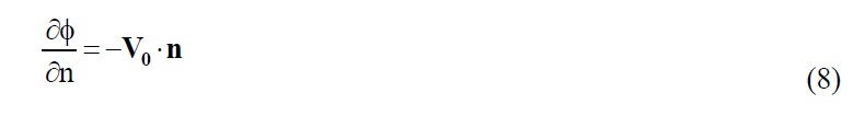
where n is the unit normal vector defined outward from the boundary surface S=∂Ω .

Cavity surface: Cavity surface is generally defined as follow:

γ is the cavity thickness function in non-orthogonal local coordinate system. s₁and s₂ are curvilinear directions element fitted in non-orthogonal reference system.

Dynamic boundary condition expresses the equality of the pressure on the cavity surface and vapor pressure.

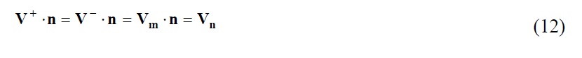
Wake surface: Wake surface is a vortex sheet with zero thickness, attached to the body and including all vortexes flowing by body. Upper and lower surfaces of the wake are shown by + and -, respectively. Wake surface must satisfy dynamic and kinematic boundary condition. To satisfy the kinematic boundary condition, vortex wake s_w should be as a surface of zero thickness. If V_n indicates the velocity of wake surface in the normal direction, then kinematic boundary condition for steady flow is:

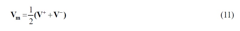
V_m is the wake average velocity of the fluid. According to dynamic boundary condition, pressure difference in two sides of wake surface is zero.

Surface at infinity: In the boundary, the surface at infinity S_∞ , disturbance caused by body and cavity surfaces tends to zero.

For the lifting problem a Kutta condition is needed at trailing edge to uniquely specify the circulation. In the present method the pressure Kutta condition is employed to determine the potential jump Δφ across the wake surface. This condition requires that the pressure difference between two sides of the lifting body at the trailing edge is zero that is (Huang et al., 2007)

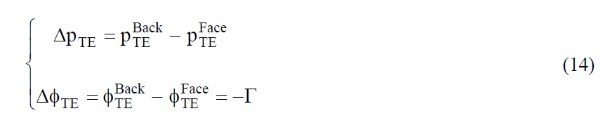
where Γ is the flow circulation for a circuit around the blade intersecting the wake at the blade trailing edge. An alternative formulation implies the calculation of φ _TE by satisfying, which means solving the non-linear equation:

φTE may be calculated both by the iterative pressure Kutta condition.

On the other hand, two boundary conditions are re-defined for propeller cavitation as follows:

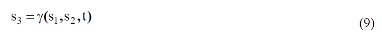
In partial cavitation, kinematic boundary condition is expressed using the material derivative concept in non-local coordinate system. For the treatment of the boundary conditions on the cavity surface it is convenient to use a curvilinear surface fitted non-orthogonal reference system (s₁,s₂,s₃ ) with unit base vectors (t₁, t₂, t₃) that t₁, t₂ are the local tangent vectors and t₃ is the local normal vector.

Cavity surface is not known and to determine it, dynamic and kinematic boundary condition should be investigated. Let F(s₁,s₂ ,s₃ , t ) = s₃ − γ(s₁ ,s₂ , t) = 0 the cavity surface equation. Then the kinematic boundary condition states that the cavity surface should be a material surface of the flow:

We get for the velocity components,

And the definition of a gradient ∇of the form,

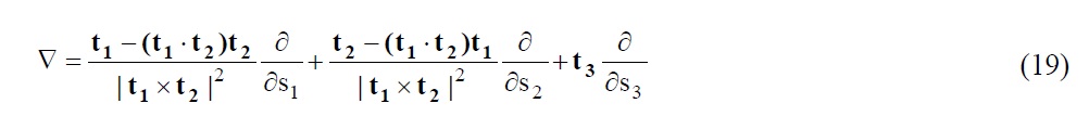
Eqs. (18) and (19) can be combined to form the same material derivative operator in the non-orthogonal reference system as follows,

’is the angle between the non-orthogonal tangent unit vectors t₁ and t₂. The KBC can therefore be written as,

Eq. (21) is a linear partial differential equation for γ . The resultants of this equation are the values of cavity thickness or cavity height.

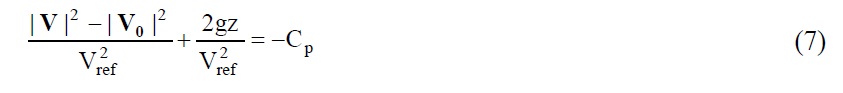
The dynamic boundary condition Eq. (7) is formulated taking into account Eq. (10):

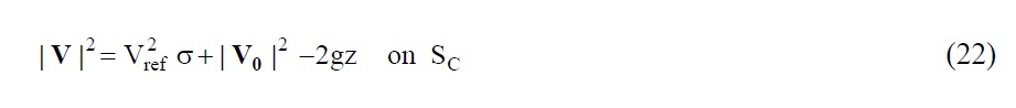
In the non-orthogonal reference system, this equation is:

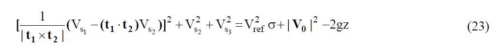
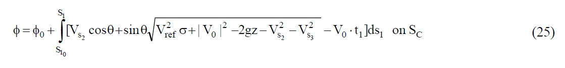
The dynamic boundary condition is non-linear on φ due to the presence of quadratic terms on the perturbation potential spatial derivatives. Dynamic boundary condition may be changed to Dirichlet boundary condition on φ . So, for V_s1 , the following equation is obtained.

By integrating along s₁ from flow detachment point, s₁₀ = s₀ , and considering the potential value φ, following equation is extracted for φ .

Velocity potential in fluid domain Ω is obtained using classic integral. Based on Green’s third identify equation φ can be written as

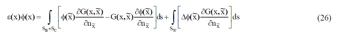
where x a point in fluid domain is Ω,

is a point on the boundary surface S = ∂Ω ,

is normal vector in

and ’(x) is a constant value which depends on the position of field point x .

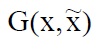
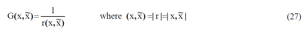
is a proper Green’s function for a 3-dimensional analysis of fluid flow that defined as:

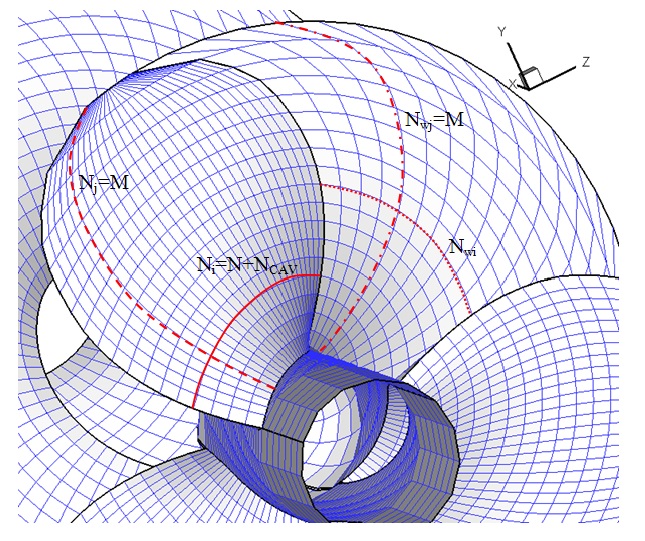
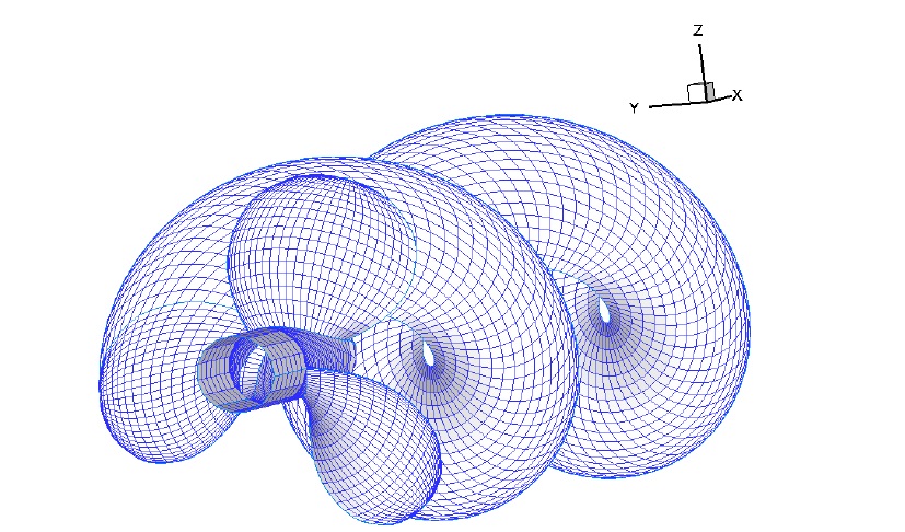
In the state of partial cavitation, the total number of elements is equal to those of the body. Figs. 1 and 2 shows the number of elements, cavity zone on the propeller and trailing vortex wake. The discrete form of integral equation (26), in the steady state condition and uniform inflow is:

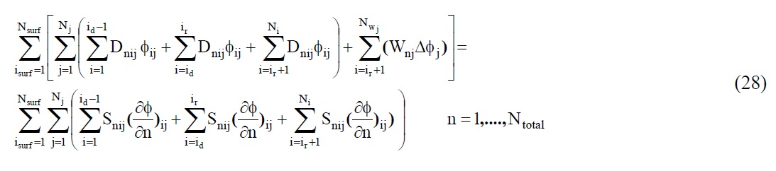
The indices i , j and n map quantities to panel elements. n is control point and i , j (or m ) denote location of field point. i_surf is the index of analyzed surfaces (back-face blades and wake surface), N_i is the number of divisions in the direction of blade chord, N_j is the number of divisions in the radial direction of the blade, N_wj is the number of wake panels, i_d is the index of element in the direction of chord in which cavity detachment occurs, i_r is the number of element in the chord direction in which the cavity surface gets closed, N_cav = i_r − i_d + 1 is the number of elements under the cavitation in chord direction. The influence coefficients matrices are D_nij = D_nm , S_nij = S_nm , W_nij =W_nm respectively for the body dipoles, body sources and wake dipoles. They are defined as:

Considering the discrete form of Eq. (26), the algebraic linear equations system is constructed, and then the unknown values matrix ( φ ) is extracted. In first step cavity end points obtained based on the pressure distribution from the fully wetted analysis of propeller. This means that each element has a pressure less than or equal vapor pressure extraction and end points can be estimated.

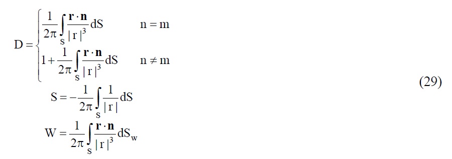
From the general dynamic boundary condition for the cavity surface, the potential of the cavity is prescribed as the sum of the detachment point potential φ₀ with a term that depends on the cavity surface potential

The potential on the cavity is then prescribed by

The various choices for location of the detachment point were analyzed and point of minimum pressure is selected. This point is considered to be set on a boundary point of a panel instead of a center point, and it is the first point of the cavity part and the last of the wetted part. This means that its potential value ensures continuity of the potential between the wetted and the cavity parts of the body. Its value is calculated based on the values of the wetted part adjacent points by means of an extrapolation:

The order of the extrapolation scheme used is Jext . In present study Jext = 2 .

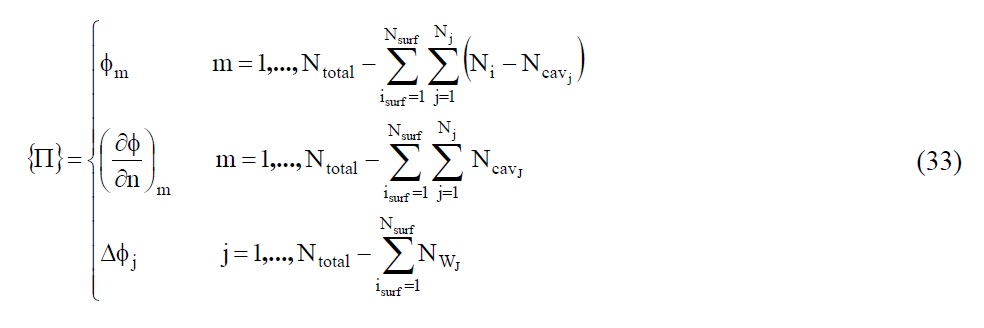
Setting the unknown terms on the left hand side of the system and the known terms on the right hand side, Eq. (28), yields

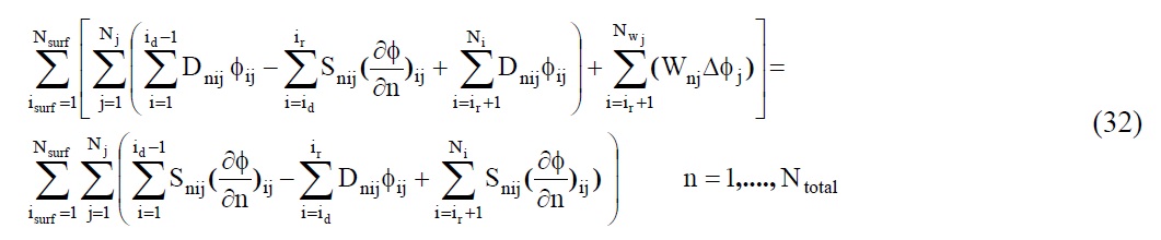
The linear system of equations can be written as:

[LHS]{ Π } = {RHS}

That { Π } as follow:

The total forces and moments acting on the propeller are evaluated by integrating the pressure coefficients over the propeller surface. The pressure component of thrust and torque of propeller are expressed as follows:

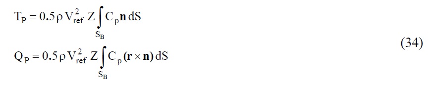
where Z is the number of blades and ρis the density of fluid. The contribution of the viscous forces is given by

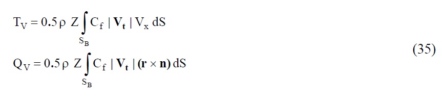
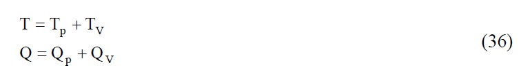
whereC_f is the local skin friction coefficient that is calculated from two-dimensional boundary layer theory. Consequently, the total thrust and torque of the propeller are obtained as

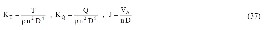
The non-dimensional hydrodynamic coefficients (thrust coefficient K_T and torque coefficient K_Q ) of the propeller are expressed as follows:

In order to analyze and examine the numerical results, DTMB4119 standard propeller is selected. At first, to survey the mesh independency condition for analyzing, the changes of element numbers in both chord and radial directions are investtigated. The minimum required number of elements in chord and radial directions shall be considered that the results do not change by variation of the elements number. Based on the present study, the optimized grid generations on propellers have much effective in analyzing the propeller in wetted and cavitation states. Data concerning pressure coefficient at different radial sections in wetted condition is determined and compared with experimental data and existing numerical researches in 20^th ITTC was held in Korea.

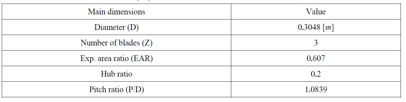
One of the most significant factors in propeller modeling is sufficient geometrical information about the desired propeller. Table 1 shows main dimensions of DTMB4119 propeller.

The method of mesh generation and wake producing as shown in Fig. 2 is one of the influential factors in propeller analysis. Because of the pressure gradients are very sensitive in blade boundary edges, cosine spacing in the chord and radial directions are used. In the boundary areas of blades, mesh density is increased and the variation of pressure distribution is better extraction.

Since the kind of applied mesh, elements type and numbers have significant effect on the accuracy of results. So first of all, the appropriate mesh should be generated to get better smooth and fair surface. After generating the geometry, one of the most important cases is evaluating the mesh independency. The mesh independency term is achieving the appropriate mesh which the results won’t significantly change with mesh refining and increasing the total element numbers. In the present study, in order to achieve the appropriate element numbers, they are changed in accordance with the chord and radial directions .

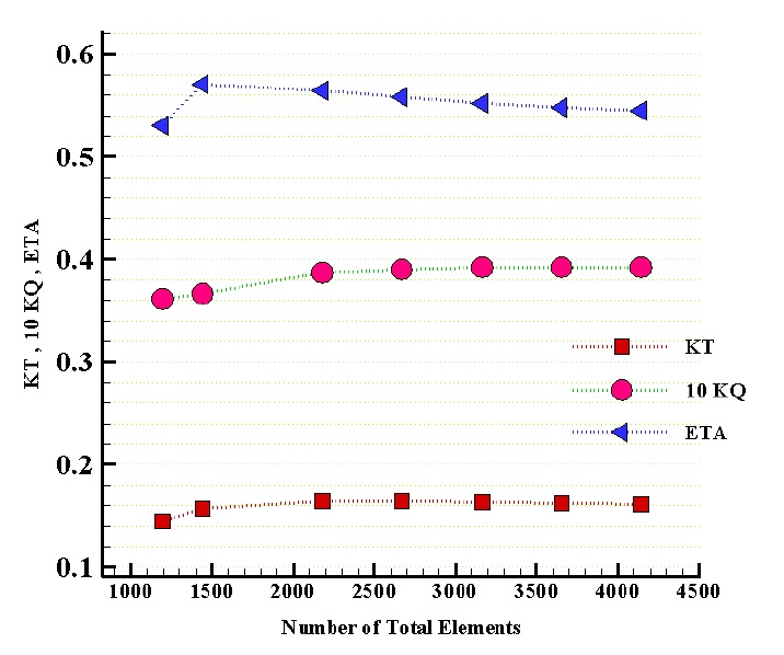
In Fig. 3, the mesh independency has been evaluated in accordance with the total element numbers and no change in results. As can be seen, there is no noticeable change in thrust and torque coefficient and efficiency when the element numbers are 3500 or above. It should be mentioned that all calculations are done at advance velocity ratio (J) is equal 0.833 (J = 0.833).

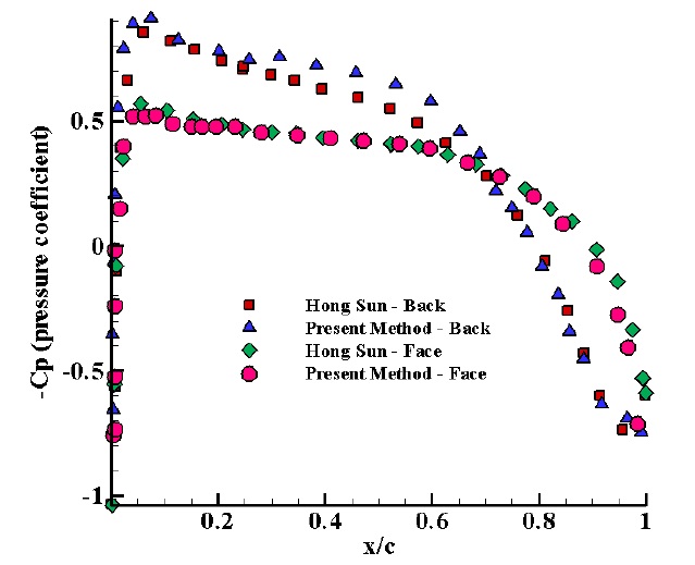
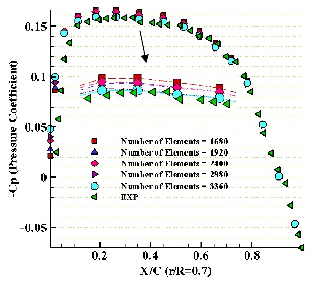
Extending the mesh independency, it is also investigated on the pressure distribution coefficient that is shown in Figs. 4 and 5. As can be seen, when the element number increases the numerical analysis results on the face side of the blade are close to the experimental data. Also, a similar result is also obtained on the back side of the blade.

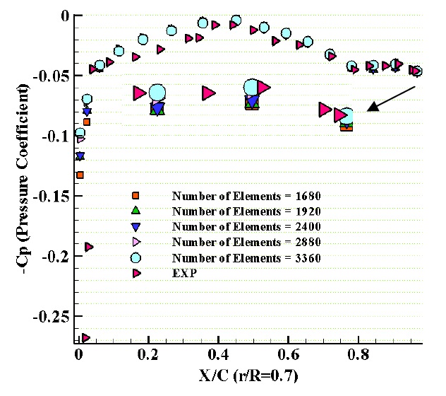
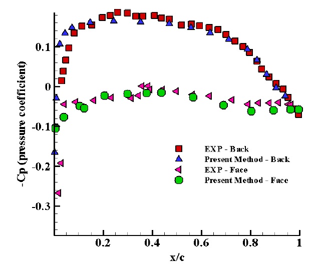
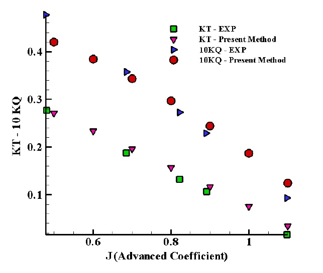
Calculations of the pressure coefficient are one of the most essential parameters for estimating the hydrodynamic performance. Fig. 6 presents the comparison of the pressure distribution on the back and face sides of DTMB4119 propeller in the section of r/R = 0.7. The present numerical results show good correlations with experimental data. Comparison of the thrust and torque coefficients of DTMB4119 propeller is shown in Fig. 7. There is a good accommodation between obtained numerical data and experimental data. Generally, the error is less than 5%. It can be interpreted in such a way that in very low advanced coefficients, considering the assumption, error increases due to low Reynolds number.

Sheet cavitation on DTMB4119 propeller in a flow condition with advanced coefficient of J=0.833 and cavitation number of σ=1.02in open water flow condition is analyzed. Physical properties of the sea water areρ =1025 kg/m³, p =101.325 Kpa, vapor pressure = 1.67 Kpa and water viscosity μ = 0.001 kg.s /m.

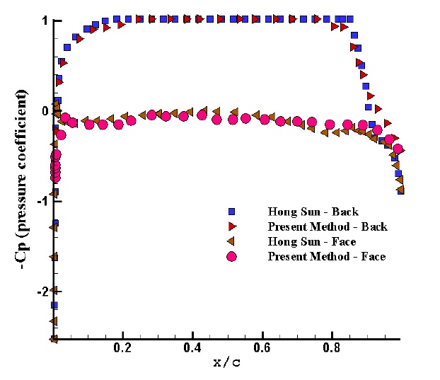
The comparison of pressure coefficients at face and back surfaces of the propeller is presented in Figs. 8 and 9 at two radius (r = 0.24 R, 0.7 R). It is shown that the comparison of the pressure is good agreement to Hong’s data (2008) at r = 0.7 R, but slightly different at r = 0.24 R.

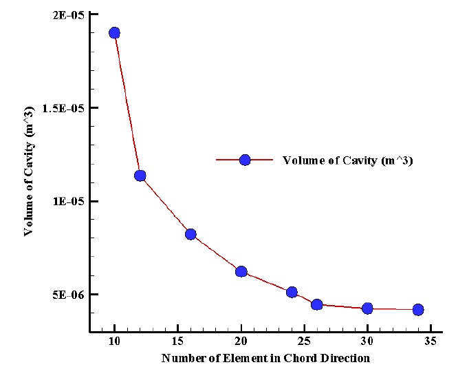
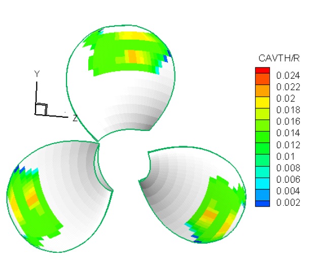
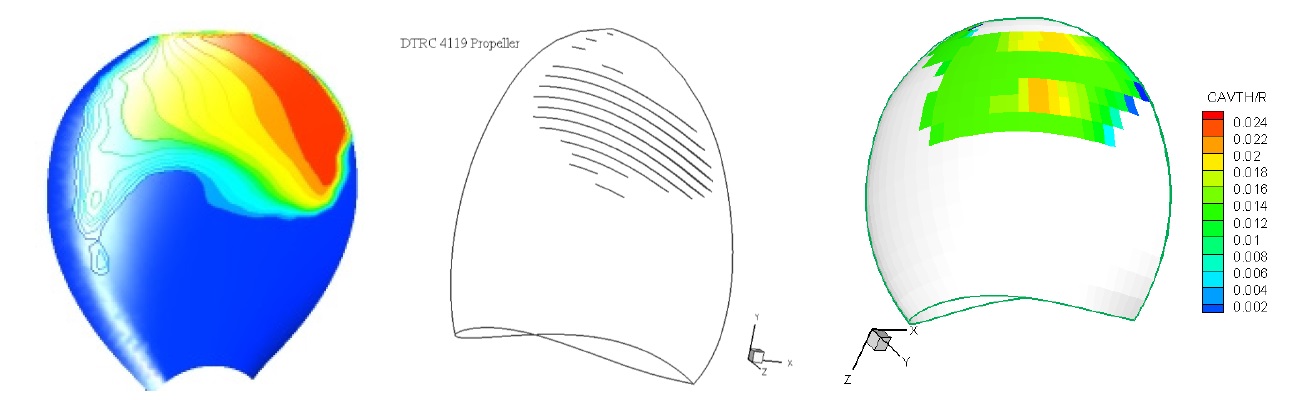
Cavity volume versus the changes of element number in chord direction is shown in Fig. 10. When the number of elements in chord direction increase the meshes become fine. Here, the cavity volume is converged by 30 elements in chord direction. On-dimensional cavity thickness contour is shown in Fig. 11 at J = 0.833 andσ=1.02. As observed in the figure, the maximum thickness is 0.025R that R is propeller radius. Fig. 12 shows the comparison of the cavity thickness on the blade surface. Right figure is shown the present method and left one is given by Hong result.

In this paper, the boundary element method is applied to evaluate the hydrodynamic characteristics of the sheet cavitating and non-cavitating propeller. Based on the numerical calculations, the following conclusions can be drawn:

The effect of number of mesh was investigated. For the present three-bladed propeller, the number of 3500 meshes may be enough for the calculations.

Pressure distribution coefficients as well as the thrust and torque coefficients are determined in both cavitating and noncavitating conditions on propeller blade. They are in good agreement with experimental data.

The cavity thickness determined by the present method is compared and have good correlation with available data.

Based on the obtained data it can be seen that there is a good match between the thrust coefficients and the propeller torque without cavitation with experimental data. As it can be shown from the grid optimization, the data has a desirable accuracy with appropriate low grid number.

Since the detachment point potential is extrapolated from the previous point in wetted area as a function of order 2 and there is a continuity between wetted and cavitation area so it can be seen that there is no sharp fluctuations and instability in the solution of the pressure distribution results and there is a good agreement between the present study pressure coefficient and empirical results in the case of cavity propeller.

In present study according to the results of vapor volume fraction contours, the effect of cross flow on cavity surface and vapor volume determination has a better agreement between the numerical results gained from the present method and fluent results than Hong (2008) result. The Slight error rate near the tip blade is owing to the lack of tip vortex modeling.

The derived vapor volume fraction, using the present method has the error of less than 8 per cent in comparison with FLUENT results and converged to a constant.

At last with considering the flow detachment point and the cross flow effect it can be seen that the data obtained from the present method (such as pressure coefficient, thrust coefficient, torque coefficient, efficiency, vapor volume fraction and cavitations area) to analyze the layer cavitation on the propeller, using the boundary element method is more accurate and has less grid than the FLUENT and Hong (2008) results.