The resonance power buoy is a convincing tool that can increase the extraction efficiency of wave energy. The buoy needs a corresponding draft, to move in resonance with waves within the peak frequency band where wave energy is concentrated. However, it must still be clarified if the buoy acts as an effective displacement amplifier, when there is insufficient water depth. In this study, the vertical displacement of a circular cylinder-type buoy was calculated, with the spectrum data observed in a real shallow sea as the external wave force, and with the corresponding draft, according to the mode frequency of normal waves. Such numerical investigation result, without considering Power Take-Off (PTO) damping, confirmed that the area of the heave responses spectrum can be amplified by up to about tenfold, compared with the wave energy spectrum, if the draft corresponds to the peak frequency, even with insufficient water depth. Moreover, the amplification factor of the buoy varied, according to the seasonal changes in the wave spectra.
Wave energy extraction makes up a renewable energy sector, and its commercialization and real sea verification are being actively performed worldwide. Its most studied area is the point-absorber-type hydrokinetic power system. The absorber-type hydrokinetic energy extraction equipment normally uses a buoy, which is called a
There have been many researches regarding the performance of a point absorber as wave energy converter since 1970s. Mostly, they take advantage of large resonant motions of a floating buoy and the electricity is generated by hydraulic PTO system or linear generator system. Budal and Falnes (1975), French (1979), and French and Bracewell (1995) studied a small heaving buoy in waves for extracting wave energy. They found that energy can be absorbed from a sizable width of wave crest much larger than the diameter of the buoy if using the resonant motion of a floating buoy. Falnes (1999) proposed a two-object hydrokinetic power generation system that consisted of inner and outer buoys, and was designed to easily acquire energy, by maximizing the relative vertical motions when resonance occurred, as the natural frequency of the inner buoy corresponded
with the mode frequency of the real sea area, where the system was installed. In addition, Grilli et al. (2011) verified, through tests and numerical calculations, that the energy extraction efficiency increased from the SPAR-type buoy and three satellite buoys with different heights that were moving around the resonance area, and suggested a measure for adjusting the natural frequency of the system for the safety and resonance of the hydrokinetic power generation system, through a combination of the main buoy and satellite buoys. Kweon et al. (2013a) have proven, through a systematic experiment, that the resonance buoy was amplified up to 5.66-fold in the amplitude ratio. As a linear generator is mounted on this resonance buoy, two movers operate according to the heaving displacement amplitude in this system.
Deep sea energy production increases the cost of transporting electricity to land, and an area with relatively smaller wave energy causes power generation economic feasibility problems. To overcome such problems, the increased displacement of the water level caused by the superposed waves that are reflected by the front surface of the breakwater installed in a small-sized fishing port can be used. However, low depth has insufficient water depth to produce resonance in the peaked frequency band, where the wave energy is concentrated. Therefore, the amplification of the heaving displacement of the power buoy must be verified. In this study, the waves that occurred during the entire period, regardless of whether or not big waves attack them, are called normal waves, and were used to investigate the resonance characteristics of the buoy.
This study investigates the amplitude effects of the heaving displacement of the power buoy, which needs to produce power constantly in low depth, where sufficient resonance depth cannot be secured, through a time-domain numerical simulation from the wave energy spectrum.
WAVE OBSERVATION AND CORRELATION ANALYSIS OF WAVE DATA BY MONTH
In this study, real sea data were analyzed, to simulate the motions of the power buoy. The analysis was performed on the heaving displacement of the superposed waves reflected by the front surface of the breakwater, as described in Section 1. As such data correspond to the normal waves, they are considered appropriate for investigating the amplitude characteristics of the power buoy, which was installed for continuous power generation.
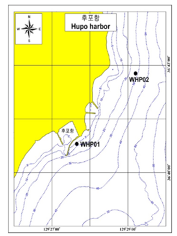
This study examines the wave data obtained around the eastern and northern coasts of Hupo Port in Uljin-gun, Gyeongsangbuk- do, South Korea (see Fig. 1), by using a wave and tide gauge (WTG). The wave observation started at the designated point, WHP01 (129°27’40”E, 36°40’35”N, with a water depth of about 10
For the data analysis, first, the pressure data that were measured continuously at 0.5
>
Correlation analysis of the wave data by month
To design the resonance power buoy for electric power production, the wave period and wave height variations have to be predicted, to set the dimensions of the power buoy according to the target power production. However, multiple numbers of power buoys are needed for areas where the seasonal period and the wave height variations are distinct, and the power buoys must be installed based on such predictions. Meanwhile, separate examination of each monthly period would require 12 power buoys with different dimensions, which is economically unfeasible. In addition, the extraction efficiency of one buoy may differ depending on the seasonal period, and the difference in the wave height. That is, as the regional factors of the seasonal waves dominantly affect the extraction efficiency, rather than the performance of the power buoys, they create a problem with the design.
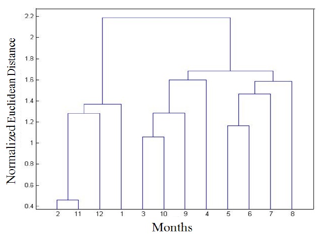
Considering the aforementioned problems, in this study, the buoy dimensions that caused the waves to be separated from the seasonal wave variations according to their similarity were determined, and the extraction rate of each corresponding wave was calculated separately. To achieve these, a relative correlation analysis was conducted in areas where the variations in the seasonal wave characteristics were comparatively distinctive. To investigate the correlation of waves all year around, the observation data that were obtained in the real sea located at 129°27’40”E, 36°40’35”N with a water depth of about 10 m for about three years from May 2002 to March 2005 were analyzed.
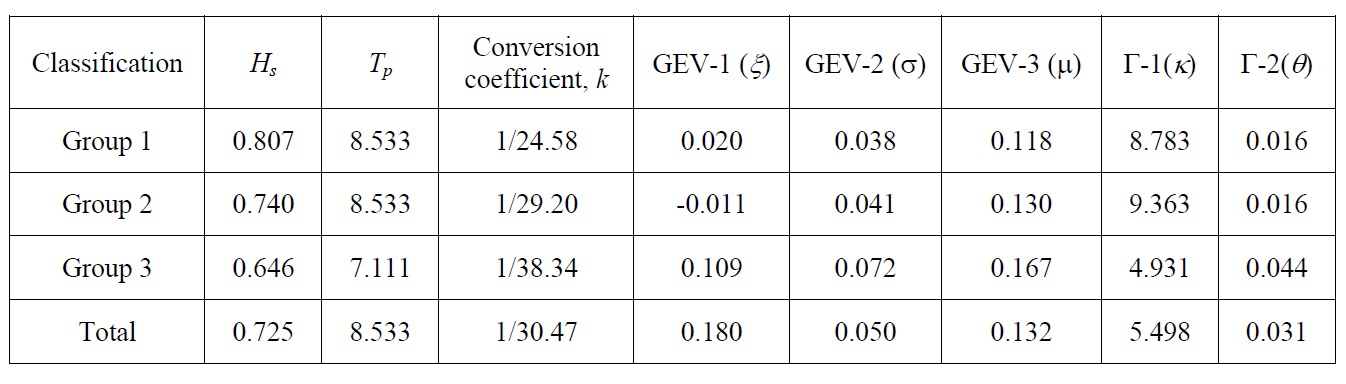
The wave characteristic data were divided into the monthly data (that comprised a total of 12 sets); the information on the wave height, peak period, average and estimated wave force of the divided data were normalized (mean = 0 and variance = 1), as shown in Table 1; a cluster analysis was conducted on the normalized data using the Euclidean distance (the mathematical distance of the normalized information), without assigning the weighted value number according to the correlation of the data; and the data were reconstructed into three sets of clustered data. The constructed data were regrouped into Group 1 (the data for November, December, January and February), Group 2 (for March, April, September and October) and Group 3 (for May, June, July and August).
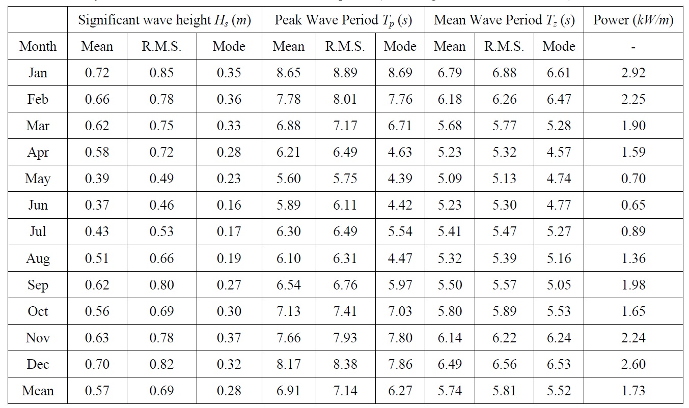
Monthly variations in the wave characteristics and power (according to Kweon et al., 2013b).
SPECTRUM ANALYSIS BASED ON CORRELATION ANALYSIS
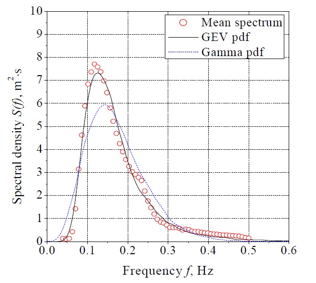
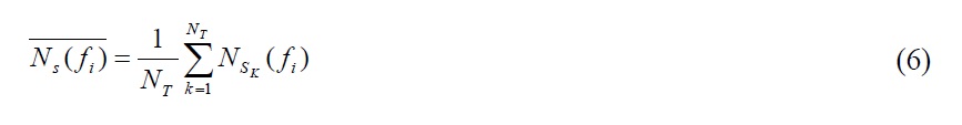
The wave observation was discontinuously conducted at certain intervals in the real sea area. Therefore, the frequency spectrum can be analyzed using the time series data on the water level elevation for each data set, and this study intends to obtain the mean spectrum for all the data sets. The mean spectrum can be obtained using this method: the corresponding frequency energy according to each frequency for the entire set is aggregated, divided by the number of sets, and applied to the whole frequency-domain. The mean spectrum of the estimated spectrum
where,
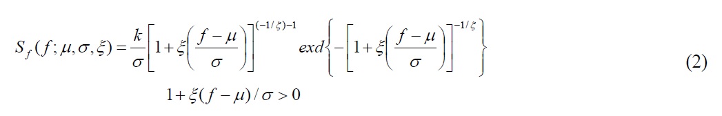
To express the normal wave spectrum, the Generalized Extreme Value (GEV) Cumulative Distribution Function (CDF) proposed by Kweon et al. (2013b) was converted to the probability density function (pdf), and the following equation that is marked with the conversion factor was used:
where,
where, the subscript
On the other hand, the Gamma PDF, which was selected as another spectrum function candidate, is described in the following equation, which is expressed with two parameters:
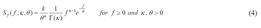
where,
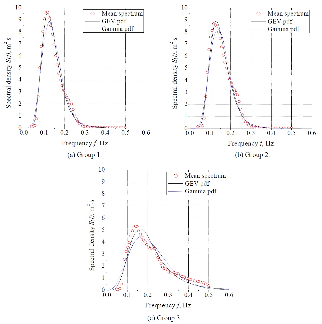
The group-averaged spectrum was calculated using the clustered data described in Section 2, and the parameters of the GEV and Gamma functions were estimated for each mean spectrum. The estimation technique was used with the maximum likelihood method, and the estimated parameters are presented in Table 2. On the other hand, the wave information such as the significant wave height and the peak period was deduced from the mean spectrum of the classified data.
[Table 2] Parameter estimates of the normal wave spectrum.

Parameter estimates of the normal wave spectrum.
COMPARISON AND ANALYSIS OF THE POWER BUOY MOTIONS
The dimensions of the resonance power buoys can be easily decided from the wave frequency spectrum for the design resonance frequency. However, the existing spectrum types have limits in expressing the normal waves, and in this study, the mode frequency spectrum of the waves that were observed year-round was analyzed. The resonance frequency of the power buoy was selected from the mode frequencies of the generated waves, and used to decide on the draft, from among the buoy dimensions. To compare and analyze the influence according to the spectrum type of the incident waves, the heaving motions of the numerical model buoy were calculated as examined by Kweon et al. (2013a). In this study, the reductions in the motions of the buoy due to actual PTO system by linear generator were not considered. The effect of actual PTO system on the motion of a floating buoy has been investigated by Cho et al. (2012).
>
Estimation of the mode frequency spectrum
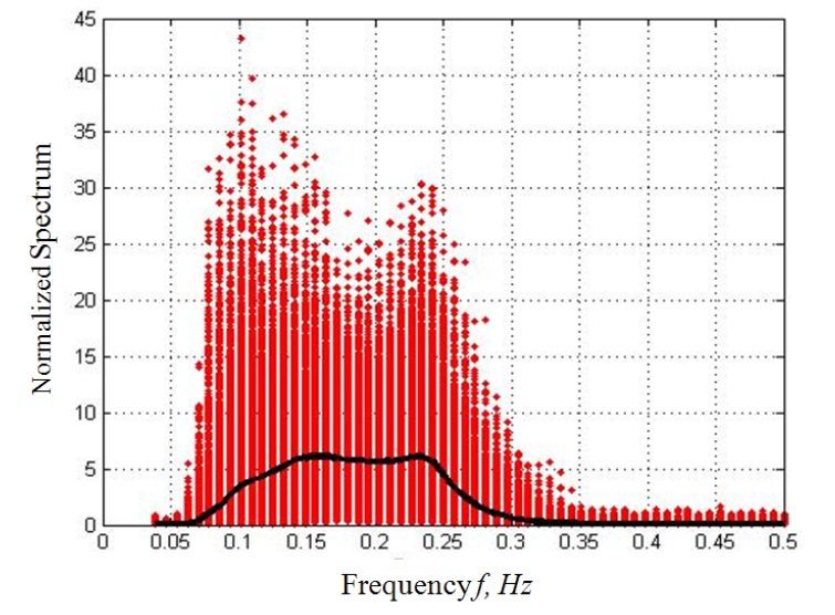
For maximum power extraction, the corresponding resonance design according to the peak frequencies in Fig. 2 is required; but an examination would be needed to decide on the design resonance frequency, as the mode and peak frequencies of the normal waves are different, as shown in the results of the study of Kweon et al. (2013b). The mode spectrum estimation differs from the arithmetic mean, because it is based on the occurrence frequency of the spectrum. To retain each observed spectrum, even from the aspect of the frequency of occurrence, the spectrum size was normalized as follows, by dividing it by the spectrum surface:
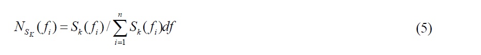
where,
where,
The normalized spectrum appears as two mountains, the representative values of which can be connected with the black line as shown in Fig. 5, while considering the spectrum as the density of the spectrum. The variations in the representative values show a flat shape between the frequencies of 0.15
>
Decision on the power buoy dimensions
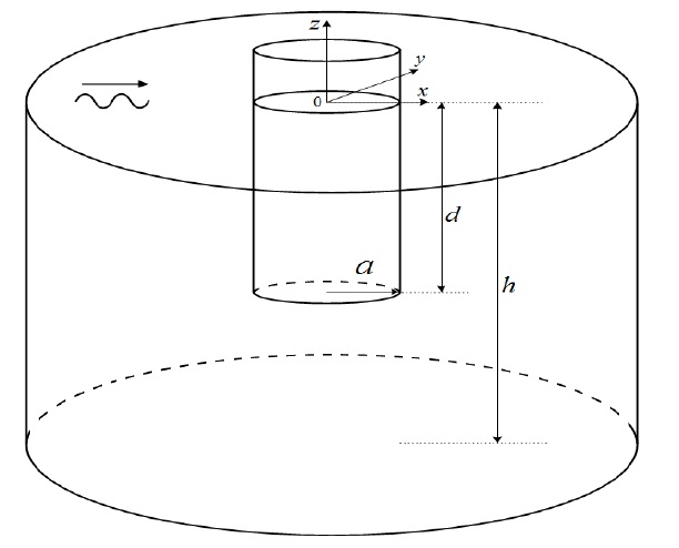
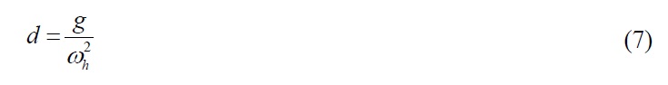
The power buoy is an effective wave-power extraction device that uses the resonance phenomena with incident waves. Therefore, for effective extraction, the buoy must be designed so that the natural frequency may coincide with the peak frequency of the incident wave spectrum. The draft (
where,
Had the natural frequency of the power buoy been designed to coincide with the peak frequencies of the normal wave spectrum in Groups 1, 2 and 3, the power buoy drafts would have appeared as 20.02, 15.32 and 10.64 m in each group, respectively. However, as the power buoy was installed at point WHP01 in low depth (less than 10
[Table 3] Specifications of the power buoy.

Specifications of the power buoy.
>
Motion response of the power buoy
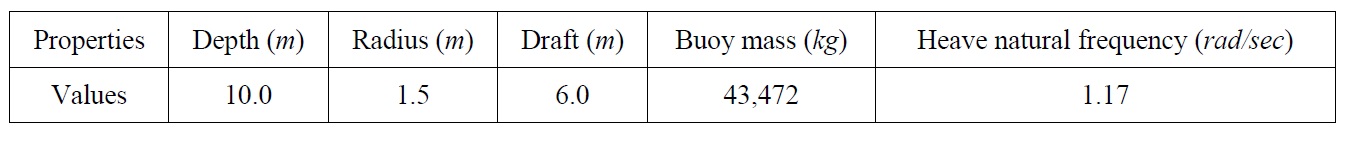
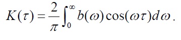
To investigate the amplification effects of the heaving motions when the power buoy was tuned to resonance with the incident waves, a time-domain motion analysis was conducted on the normal-wave-spectrum Groups 1, 2 and 3 proposed in the previous section. The hydrodynamic force (added mass, radiation damping coefficients) and wave exciting force of the power buoy that were needed to conduct the time-domain analysis were calculated in the frequency-domain, and the commercial AQWA code based on the boundary element method was used in this study. As the viscous effects were not considered in the commercial code, the viscous damping coefficient (
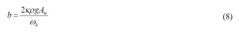
where,
Fig. 7 shows the results of frequency-domain analysis for the models presented in Table 3. Each graph represents the Response Amplitude Operator (RAO), wave exciting force, added mass and radiation damping coefficient of the heave motion. As shown in Fig. 7(a), the buoy tends to follow the waves as the frequency decreases; the RAO ( =|
The time-domain equation for the heaving motion of the power buoy was derived from Newton’s second law, and can be described as follows.

where,
>
Comparison of the heave RAO of the power buoy
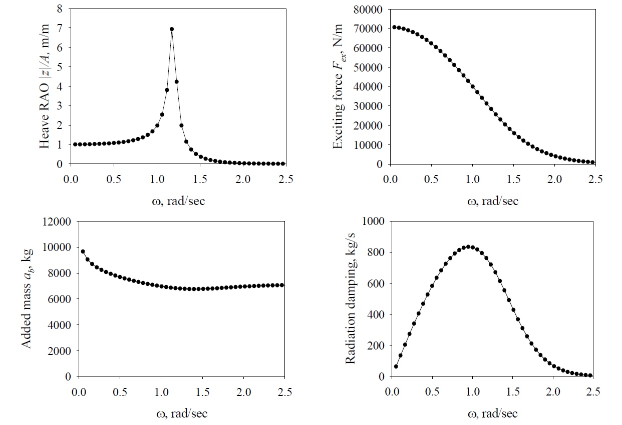
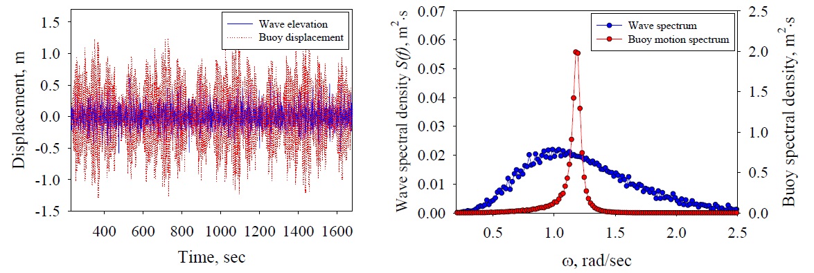
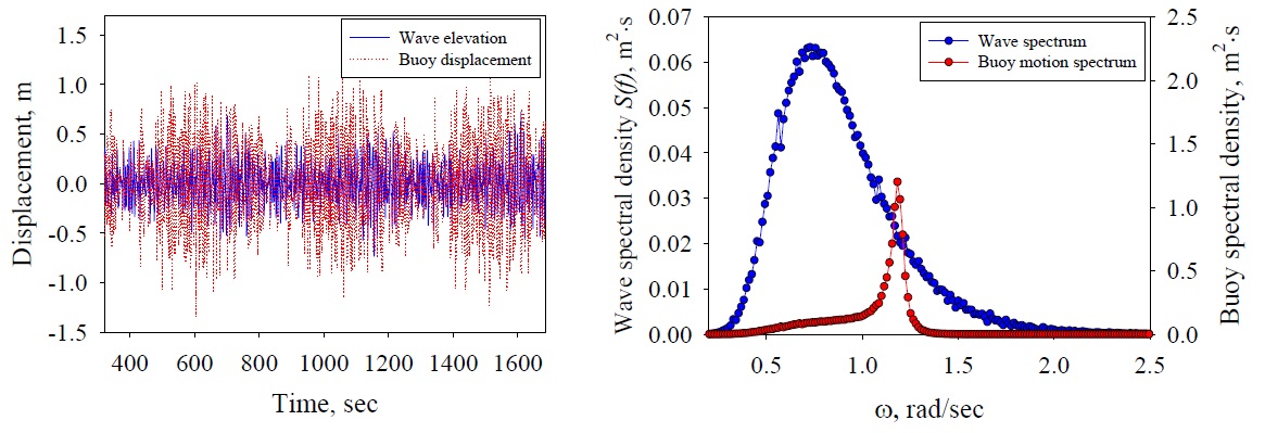
The results of the time-domain analysis for the normal-wave Groups 1, 2 and 3 spectra described in Chapter 3 are presented in Figs. 8-10, respectively. Figs. 8-10(a) show the time series data on the wave elevation and heave motion of the buoy for the normal-wave Groups 1-3 and Figs. 8-10(b), the spectra obtained from applying the Fast Fourier Transform (FFT) technique on the time series data. Groups 1-3 showed that the heave motion of the power buoy tuned to resonance with the incident waves were largely amplified. To calculate the representative values (SWH: significant wave height and SBH: significant buoy height) in irregular waves, the SWH and the SBH of the power buoy were calculated by applying the zero-crossing method to the time series data. In addition, the energy volumes (WSA: wave spectrum area and BSA: buoy spectrum area) of each group were arranged by integrating the area of the spectra in Table 4. Group 1 showed that SWH is equal to 0.7714
[Table 4] Statistical properties of irregular waves and theirbuoy motion.
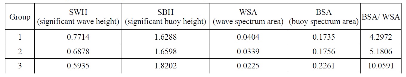
Statistical properties of irregular waves and theirbuoy motion.
The use of a resonance buoy to improve the efficiency of wave energy extraction is becoming popular. In this study, wave observation data were used as the input conditions, for the answer to the question as to whether or not the resonance effect was still effective in low depth, where a sufficient resonance draft that was appropriate to the peak frequency of the observed spectrum was not secured. Therefore, in this study, the heave motion characteristics of the buoy were investigated when the buoy is resonated with incoming waveswithhigher frequency than the peak frequency of the observed spectra in a real sea area. The higher resonant frequency corresponded to the case with a smaller buoy’s draft. The following conclusions were obtained.
(1) A new expression utilizing the Probability Density Function (pdf), based on the Generalized Extreme Value (GEV) Cumulative Distribution Function (CDF) for the normal wave spectrum, was proposed.
(2) The circular cylinder-type buoy with a draft smaller than the resonance draft that corresponded to the peak frequency in the real sea area, produced larger heaving displacement spectra, than those of the entire incident wave energy.
(3) The amplification rates of the buoy varied, as the wave spectra changed by season.
(4) The changes in the wave spectra by season affected the areas of the heaving displacement spectra of the power buoys with the same dimensions, so many other buoys with different resonance drafts had to be installed, for smoother energy production.
(5) For the optimum design of the power buoy, the buoy motions must be analyzed, while considering the PTO-damping items in low depth.