This paper presents a MAAP4 based analysis to examine the sensitivity of a key metric, in this case hydrogen production, to a set of model parameters that are related to the Level 2 PRA analysis. The Level 2 PRA analysis examines those sequences that result in core melting and subsequent reactor pressure vessel failure. The analysis assessed this sensitivity for loss of balance of plant (LBOP), loss of offsite power (LOOP), and small loss of coolant accident (SLOCA) events identified by AREVA Inc. as the Risk Dominant Scenarios for a Babcock & Wilcox (B&W) nuclear plant as defined by the U.S. Nuclear Regulatory Commission1. The analysis identified the relative importance to hydrogen production of individual contributors and MAAP4 model parameters. Hydrogen generation was chosen as the matrix because of its direct relationship to oxidation. The higher the oxidation the more heat is added to the core region and the faster the relocation (core slump) should occur. This, in theory, should lead to shorter failure times and subsequent “hotter” debris pool on the containment floor.
The set of parameters, and their ranges, used as inputs to the uncertainty analysis in order to quantify the relative importance of individual contributors were selected based on information provided in the MAAP Zion Parameter File2 and Reference 3.
By executing a sufficient number of variation calculations in which the uncertainty parameters are each randomly sampled using a Latin Hypercube sampling technique over their specified uncertainty range, this analysis generated coverage of the range in possible production (including the maximum) of oxidation with the reactor pressure vessel (RPV), i.e. hydrogen mass.
A single variation calculation is defined as a collection of random samples for the selection of parameters that are being analyzed. Each element of the collection corresponds to a random sample over the range of the parameter. As an example, consider the collection of parameters A, B, and C. The possible range of each parameter is imagined as 1 to 10 for parameter A, -1 to 1 for parameter B, and 100 to 200 for parameter C. Therefore, one example of an element would be a value of 5 for parameter A (a random sample over the range 1 to 10). The second element of the collection could be -1 for parameter B (again a unique random sample over the range -1 to 1). The remaining element of the collection could be 195 for parameter C (also an independent random sample over the range 100 to 200). Therefore, the collection would consist of elements A=5, B=-1, and C=195.
This collection is then used in a single MAAP calculation to define a single variation calculation. This process is repeated to provide a sufficient number of calculations to result in a statistical approximation of those elements that significantly impact the hydrogen production.
The number of MAAP4 variation calculations executed is taken to be 100 calculations for each of the Risk Dominant Scenarios in order to achieve a best estimate plus uncertainty result at a 95/95 probability/confidence level (see Table 1). The Risk Dominant Scenarios are Loss of Balance Of Plant (LBOP), Loss Of Offsite Power (LOOP), and Small break Loss Of Coolant Accident (SLOCA) sequences.
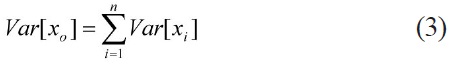
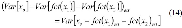
The objective of the analysis described in this section is to define and evaluate a useful statistical measure that both identifies important phenomena and quantifies the contribution of those modeling parameters to a particular output variable. The preferred importance measure is the standard deviation, σx, since it provides meaningful information about the results in terms (i.e., units) of the particular analysis measure; however, the more convenient form for statistical analysis of the standard deviation is the variance which is simply the square of the standard deviation, i.e.,
Given a best-estimate predictor model such as
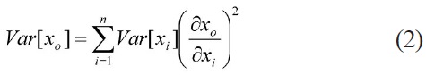
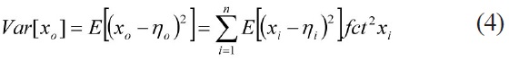
Parameters such as heat transfer, power, and break area are treated as mutually independent random variables. If all of the individual contributors are mutually independent, the partial derivative term in Equation 2 becomes zero leaving Bienayme’s equality4:
Given in terms of the Expected Value, the variance is expressed as5:
where
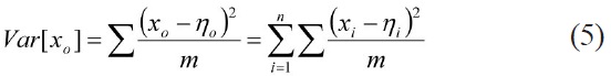
Here, Σ
The task of quantifying the uncertainty contribution of specific model parameters requires a decomposition of the total variance measure. This can be accomplished through the evaluation of a multiple-regression model. A multipleregression model simply extends the application of curvefitting to multiple variables. The main assumption applied in this exercise is that there exists a linear relationship between the dependent variable,

Each function, e.g.,

A direct solution for the regression coefficients in the multiple-regression model can be evaluated by applying least-squares techniques; however, for this application, successive evaluation of the model is necessary because the limited data sizes provide only limited information useful for resolving the model. In addition, the successive evaluation approach allows for choice among possible estimator functions derived from the least-squares technique.
The initial tasks required for this approach are defining a measure useful for identifying the importance of sampled model parameters and a measure for identifying when the usefulness of the data for resolving the model is exhausted. With regard to the first measure, several rank and correlation expressions from sensitivity analysis are available, such as the Standardized Rank Regression Coefficient, Rank Correlation Coefficients, and Correlation Ratios. The “Rank” methods mentioned previously replace the data with the corresponding ranks. This transformation inherently removes information from the data and is, therefore, not the optimal choice.
In contrast, the sample Pearson correlation coefficient6,
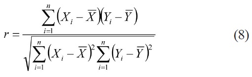
Microsoft’s® Excel computer program (referred to as EXCEL) can be used with the function CORREL or PEARSON to compute the sample Pearson correlation coefficient (
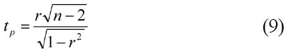
The desired result is a Pearson correlation coefficient threshold,
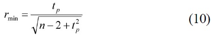
The number of samples,
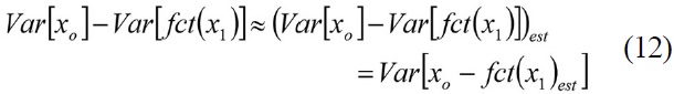
With the selection of the Pearson correlation coefficient and the identification of the “threshold of usefulness”, the procedure for quantifying process and phenomenological importance can proceed. The initial important sampled model parameter is identified by the largest correlation between the sampled model parameters and the dependent analysis measure, assuming there is at least one above the threshold of usefulness. The value of the variance of that first individual uncertainty contributor can be estimated from the error between the output variable of interest and the curve-fit estimate derived for the first individual uncertainty contributor against the output variable of interest. The result is:

where
Of course, the importance measure is a standard deviation. Following the evaluation of the variance, the standard deviation is determined from the square root. This is to be interpreted as the sensitivity of the dependent variable over the variation of a particular sampled model parameter. Further resolution of the independent sampled model parameters continues following the same procedure with the dependent variable transformed by the functional estimates of the previously evaluated important sampled model parameters. For example, the variance of the second important sampled model parameter considered, based on the highest Pearson correlation coefficient, is:
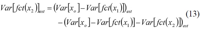
where
This calculation continues until no result within the set of correlations between the specific uncertainty contributors and the analysis measure exceeds the threshold of usefulness. At this point, the remaining variance cannot be further decomposed without significant and immeasurable degradation in precision of the results. It is possible to reveal greater resolution by adding more data through more sample calculations or a new analysis that introduces certainty for the dominant uncertainty contributors. Table 2 summarizes the sampled model parameters.
The statistical approach recommended in the performance of the severe accident analysis is based on the principles of non-parametric statistics. The process involves “Monte Carlo”-like simulations using the MAAP 4.0.7 computer code and the selected plant model developed by AREVA Inc. For each execution of the MAAP 4.0.7 code, each of the important plant process parameters being treated statistically is randomly sampled based on a linear probability distribution within an evenly distributed bin. Each execution of MAAP 4.0.7 can be viewed as the performance of an experiment with the experimental parameters being the important phenomena and plant process parameters. The result produced from each experiment can be any calculated measure such as hydrogen concentration, containment pressure, and fission product mass. This process can treat a large number of uncertainties simultaneously, far more than could be reasonably considered with response surface techniques. In essence all quantifiable uncertainties are treated at the conditions corresponding to the severe accident calculation being performed. Unlike response surface methods, which often produce probability distributions for conditions not necessarily corresponding to the real case, this Monte Carlo “binned” method propagates input and model uncertainties at the point being analyzed.
With common response surface methods, given a large number of parameters being considered, a large number of calculations must be described and executed to cover all the various combinations of the parameters. From the results of these many calculations, a distribution of outcomes can be determined and a probability of coverage defined. The penalty of this approach is the need for a very large number of simulations to define the distribution well enough to quantify a particular coverage limit. For severe accident analysis it is impractical to perform the many long term simulations that are required. Further, this process, which results in defining a full probability distribution for several outcomes of interest, provides more information than is needed, because sufficient insight into severe accident response can be found by examining an outcome approaching the tolerance limit of all possible outcomes. Ideally, the method of evaluating the statistics would reduce the number of required calculations to determine a desired probability level. As such, a non-parametric statistical approach was selected.
Starting with Wilks in 19417, non-parametric methods have been used to determine tolerance limits. Tables were created by Somerville in 19588 that have been used widely for non-parametric tolerances in a variety of applications, including regulatory guides9. Non-parametric statistical techniques are useful in situations where acceptance or rejection is based on meeting a tolerance limit and where you do not need the probability distribution itself10.
The non-parametric method follows from combinatorial theory. For a series of random samples arranged in ascending (or descending) order, the probability,
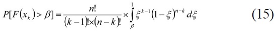
where
The term

For the case in which
The parameter of interest is

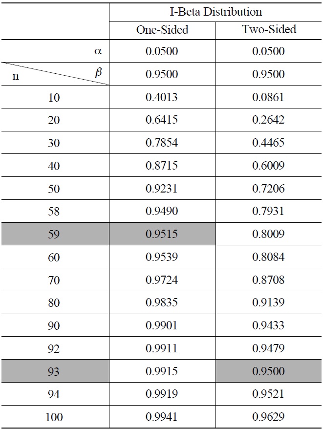
Solving for n, the solution is 58.4. If 59 observations are drawn from an arbitrary, random distribution of outcomes, then with 95% confidence, at least 95% of all possible observations from that distribution will be less than the resulting largest value; that is, this result is the 95/95 tolerance limit. Note that this conclusion is independent of the distribution.
However, there is some debate as to whether 59 samples are truly sufficient to cover the number of parameters examined in this analysis. The case for 59 observations is based on the results being treated as a one sided distribution. That is to say that one is concerned with the distribution being either below a limit on the high end of the distribution or above a limit on the low end of the distribution. This analysis is not concerned with being under or over a certain limit. This analysis is looking for the best coverage of the output variable in order to determine correlations between the input and output variables. Therefore, a two sided approach should be used.
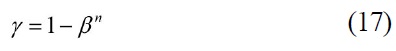
In Somerville’s model, the level of confidence (
[Table 1.] Level of Confidence (γ)

Level of Confidence (γ)
The second column of Table 1 shows the level of confidence for a one sided distribution, meaning all values are below a maximum value or all values are above a minimum value. The third column of Table 1 shows the level of confidence for a two sided distribution, meaning the values are evenly distributed on both sides of the mean. Alpha (
A Latin Hypercube sampling12, which is discussed in Section 4.3, gives better coverage than a Monte Carlo sampling. Therefore, this analysis used a Latin Hypercube style sampling. The idea of Latin Hypercube sampling is to subdivide the unit cube into
The main assumption applied in this exercise is that there exists a linear relationship between the dependent variable,
The sampled sensitivity parameters were assumed to vary randomly on a uniform scale in that the resulting increase in hydrogen production is proportionate to the value.
The input variables are mutually independent.
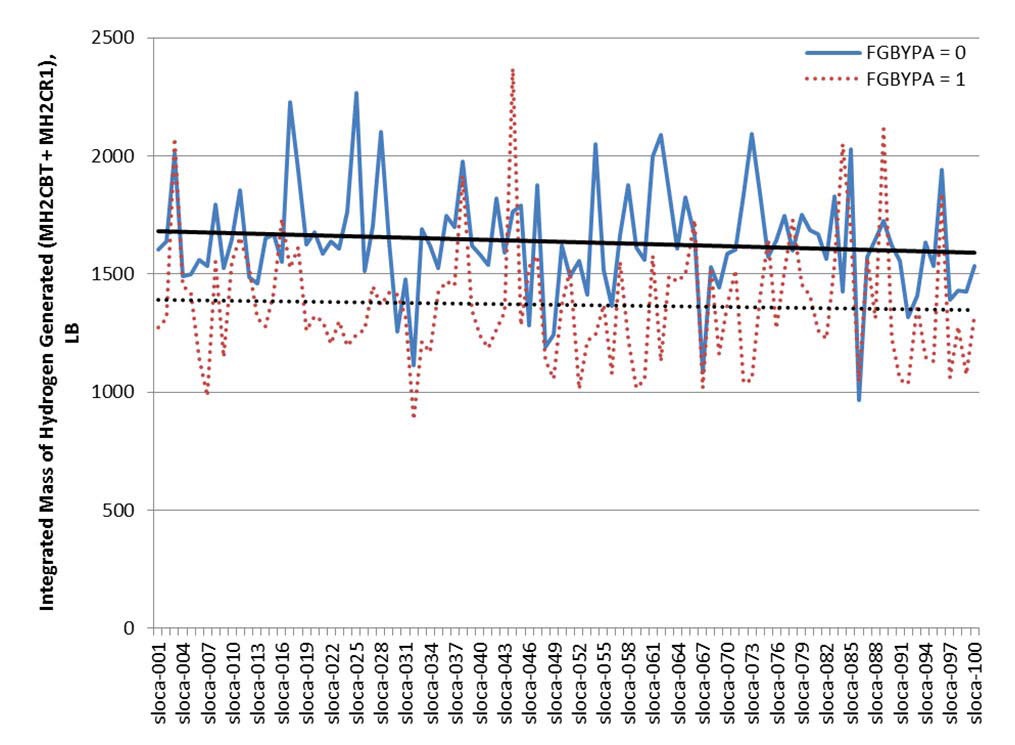
The calculation began by determining the input parameters and their corresponding ranges that affect Level 2 PRA analyses, specifically those that have the largest impact on the generation of hydrogen. The next step in this analysis was to analyze the effect the parameter FGBYPA had on hydrogen production. FGBYPA is a flag to divert gas flows in the core to the bypass channel when an entire axial row in the core is completely blocked, specifically2:
When FGBYPA=1, all channel gas flows are diverted to the bypass channel if all of the fuel channels are blocked due to a core melt progression. Once the gas is diverted, it flows up through the bypass without reentering the fuel channels. This mitigates the amount of hydrogen generated in the core due to steam upflow.
When FGBYPA=0, all channel gas flow will reappear above the blocked axial location if all of the fuel channels are blocked due to core melt progression. Upon reentering the fuel channels above the blocked row, the gas continues to travel upward through the channels. This increases the amount of hydrogen generated in the core due to steam upflow.
FGBYPA reflects a real uncertainty since the extent of gas upflow through the core or bypass around the core is a function of the porosity configuration in a blocked row, which is not well-known. Therefore, there is no one recommended sample value, and no single calculation is sufficient. Both values (0 and 1) are necessary for a proper assessment of its influence.
Therefore because of the large effect, FGBYPA was examined independently prior to performing the importance determination.
The final step was to generate the required inputs needed.
4.1 Input Parameters and Ranges Affecting Level 2 Analyses
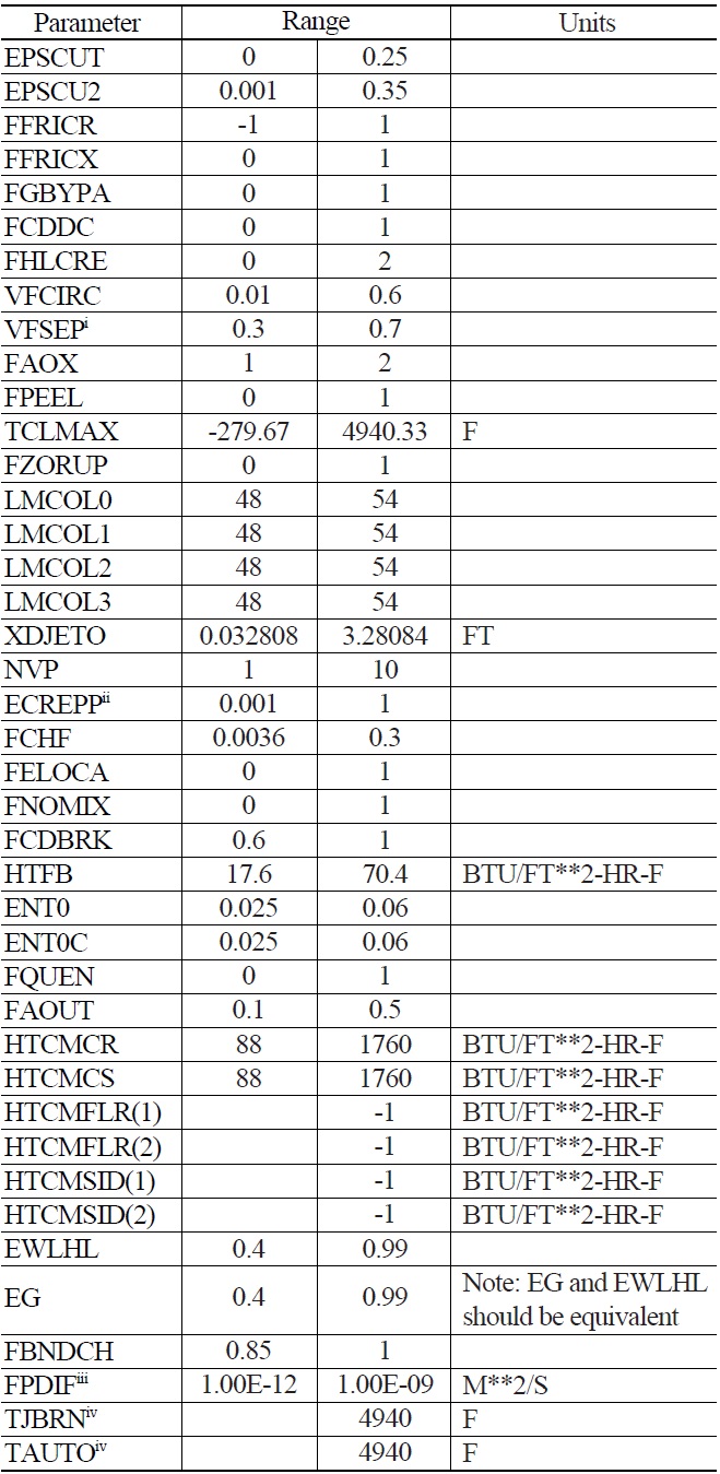
There are a number of parameters that affect Level 2 analyses. Table 2 provides a list of the parameters, and their respective ranges, that were selected for the uncertainty analysis. The set of parameters, and their ranges, used as inputs to the uncertainty analysis, were selected based on information provided in the MAAP Zion Parameter File2 and Reference 3. The uncertainty analysis quantified the relative importance of individual contributors on how they affect Level 2 analyses.
4.2.1 Parameter FGBYPA
As discussed earlier, the parameter FGBYPA is a flag to divert gas flows in the core to the bypass channel when an entire axial row in the core is completely blocked.
In the analysis of FGBYPA, the value was set to 0 for all 100 cases and set to 1 for all 100 cases of the SLOCA Risk Dominant Scenario run. Figure 1 shows the results of the FGBYPA analysis using the SLOCA Risk Dominant Scenario run. As shown, the hydrogen production when FGBYPA is set to 0 trends higher than when it is set to 1 when examining the total hydrogen at 9 hours into the scenario. Therefore, the uncertainty analysis was performed with FGBYPA set to 0, effectively eliminating any type of flow blockage.
This consequence is anticipated as it allows steam to reach the region above the blockage that would normally be steam starved.
[Table 2.] Level 2 Input Parameters

Level 2 Input Parameters
4.2.2 Parameter HTCMFLR
HTCMFLR(IC) has the same definition as the old parameter HTCMCR. However, HTCMFLR(IC) is applied to the specific corium pool IC2.
HTCMFLR(IC) also has an added feature that HTCMCR did not contain. The new feature allows the code to internally calculate the heat transfer coefficient; this is done by setting HTCMFLR(IC) to a negative value, such as -1 (this is the default). In this case, the code will implement the corium pool circulation model in subroutine HTCPOOL to determine the coefficient value.
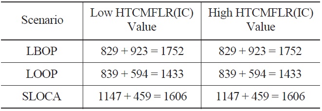
The sensitivity analysis was run to determine whether HTCMFLR(IC) had a significant impact on hydrogen production or if it was acceptable for the code to internally calculate the heat transfer coefficient by setting HTCMFLR (IC) to a negative value, such as -1. As shown in Table 3, HTCMFLR(IC) has virtually no impact on the hydrogen production (MH2CR1 + MH2CBT) using the parameter values from Set001, described in Section 4.3, for all three of the Risk Dominant Scenarios. The values for the remaining parameters were chosen based on “set001”, which will be discussed in the subsequent section.
HTCMSID(IC) has the same definition as parameter HTCMCS. However, HTCMSID(IC) is applied to the specific corium pool IC2.
HTCMSID(IC) also has an added feature that HTCMCS did not possess. The new version allows the code to internally calculate the heat transfer coefficient; this is done by setting HTCMSID(IC) to a negative value, such as -1. In this case, the code will implement the corium pool circulation model in subroutine HTCPOOL to determine the coefficient value.
In conclusion, the value of HTCMFLR(IC) was set to a value of -1 for the uncertainty analysis. Since HTCMSID (IC) has the same function as HTCMFLR(IC), it was also set to a value of -1 for the uncertainty analysis based on the supposition that since they have the same function they should behave in a similar fashion.
[Table 3.] Parameter HTCMFLR(IC) Effect on Hydrogen Production
Parameter HTCMFLR(IC) Effect on Hydrogen Production
The calculation method calls for simultaneous random sampling of the MAAP4 input parameters associated with Level 2 based on information provided in the MAAP Zion Parameter File2 and Reference 3. This random sampling generated 300 MAAP4 input files (100 for each of the relevant scenarios) to achieve an uncertainty result of greater than 95/95 probability/confidence level when applied to the best estimate hydrogen production response. Since three separate scenarios require the same input parameters, each set of input parameters were made into an include file and just the include file name was added to each input file.
The MAAP4 input files, with the randomly varied parameters located in a corresponding include file, were executed. The selection process was based on the orthogonal sampling technique.
Latin hypercube sampling (LHS) is a statistical method for generating a distribution of plausible collections of parameter values from a multidimensional distribution. The sampling method is often applied in uncertainty analysis and tends to provide more stable results than random sampling15.
The technique was first described by McKay in 197916. It was further elaborated by Ronald L. Iman, et. al. in 198117,18. Detailed computer codes and manuals were later published19.
In the context of statistical sampling, a square grid containing sample positions is a Latin square if (and only if) there is only one sample in each row and each column. A Latin hypercube is the generalization of this concept to an arbitrary number of dimensions, whereby each sample is the only one in each axis-aligned hyperplane containing it.
When sampling a function of
The maximum number of combinations for a Latin Hypercube of
For example, a Latin hypercube of
Orthogonal sampling adds the requirement that the entire sample space must be sampled evenly. Although more efficient, the orthogonal sampling strategy is more difficult to implement since all random samples must be generated simultaneously.
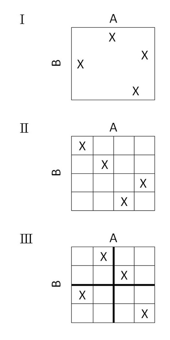
Figure 2 illustrates the difference in two dimensions between random sampling (I), Latin hypercube sampling (II), and orthogonal sampling (III); which can be further explained as:
I. In random sampling new sample points are generated without taking into account the previously generated sample points. One does not necessarily need to know beforehand how many sample points are needed.
II. In Latin hypercube sampling (LHS) one must first decide how many sample points to use and for each sample point remember in which row and column the sample point was taken.
III. In orthogonal sampling, the sample space is divided into equally probable subspaces, the figure above showing four subspaces. All sample points are then chosen simultaneously making sure that the total ensemble of sample points are a Latin Hypercube sample and that each subspace is sampled with the same density.
Thus, orthogonal sampling ensures that the ensemble of random numbers is a very good representative of the real variability, Latin hypercube sampling ensures that the ensemble of random numbers is representative of the real variability, whereas traditional random sampling (sometimes called brute force) is just an ensemble of random numbers without any guarantees.
For each case, the output hydrogen production response was extracted. The analysis to quantify the importance of the individual uncertainty parameters on the output metric of interest, i.e., hydrogen production, was then performed.
The LBOP, LOOP, and SLOCA MAAP4 scenarios were developed by AREVA Inc. for a B&W nuclear plant. The files were named as lbop-xxx.inp, loop-xxx.inp, and sloca-xxx.inp respectively where xxx represents a case number that ranges from 001 to 100. The only changes made to the input files were the case name and the addition of the include file that corresponds to each case.
The parameter ranges were subdivided into 100 equivalent sections in order to cover the entire range. A random number was then obtained for each subdivision for every variable, using EXCEL’s random number generator function RAND(), which returns a random value between 0 and 1. The random number was then applied to the subdivisions using the following equation:
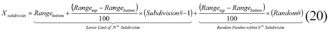
Equation 20 simplifies to:

This resulted in an ordered set of values for each parameter. In order to shuffle the ordered set of values, another set of random numbers were generated using EXCEL’s random number generator function RAND(). This set of random numbers was paired with each of the 100 subdivision values. The two were then sorted in ascending order based on the random number row. This resulted in a random ordering of the 100 subdivided values. This process was then repeated for each of the input parameters described in the following sections.
The parameter and the first subdivided value for each of the parameters were then extracted from EXCEL and placed into a text file. Each text file began with the following, where xxx is the subdivision number ranging from 001 to 100.
** Include (.inc) file for level 2 statistical analysis - Set xxx PARAMETER CHANGE
This was followed by the parameters, their values, and units if necessary, followed by an END command. Below is an example from set001.inc.
** Include (.inc) file for level 2 statistical analysis - Set 001 PARAMETER CHANGE
EPSCUT = 2.0418E-01
EPSCU2 = 1.1584E-01
FFRICR = 6.5706E-01
FFRICX = 6.8456E-02
FGBYPA = 0.0000E+00
FCDDC = 1.3852E-01
FHLCRE = 1.7835E+00
VFCIRC = 4.7642E-01
VFSEP = 3.9661E-01
FAOX = 1.6104E+00
FPEEL = 9.5471E-01
TCLMAX = 1.2533E+03 F
FZORUP = 8.2588E-01
LMCOL0 = 5.0739E+01
LMCOL1 = 4.8560E+01
LMCOL2 = 5.1444E+01
LMCOL3 = 4.9849E+01
XDJETO = 2.7707E+00 FT
NVP = 1.9701E+00
ECREPP = 2.5964E-01
FCHF = 3.4851E-02
FELOCA = 4.3695E-01
FNOMIX = 2.1044E-02
FCDBRK = 7.9346E-01
HTFB = 3.9803E+01 BTU/FT**2-HR-F
ENT0 = 4.2162E-02
ENT0C = 3.0185E-02
FQUEN = 8.6599E-01
FAOUT = 4.2418E-01
HTCMCR = 1.5044E+03 BTU/FT**2-HR-F
HTCMCS = 4.8432E+02 BTU/FT**2-HR-F
HTCMFLR(1) = -1.0000E+00 BTU/FT**2-HR-F
HTCMFLR(2) = -1.0000E+00 BTU/FT**2-HR-F
HTCMSID(1) = -1.0000E+00 BTU/FT**2-HR-F
HTCMSID(2) = -1.0000E+00 BTU/FT**2-HR-F
EWLHL = 9.3522E-01
EG = 6.1264E-01
FBNDCH = 8.8101E-01
FPDIF = 4.5137E-10
TJBRN = 4.9403E+03 F
TAUTO = 4.9403E+03 F
END
The text file was then saved as an include file. This was repeated for all 100 subdivisions and the resulting include files were named setxxx.inc where xxx is the subdivision number ranging from 001 to 100.
The input for each of the Risk Dominant Scenarios was changed by adding the following, where xxx is the subdivision number ranging from 001 to 100 mentioned previously.
include ../setxxx.inc
Each file was then saved as an input file. This was repeated for all 100 subdivisions and the files were named lbop-xxx.inp, loop-xxx.inp, and sloca-xxx.inp where xxx is the subdivision number ranging from 001 to 100.
An LBOP event can be caused by a failure of the Normal Heat Sink, Circulating Water System (cooling water to the condenser), Auxiliary Cooling Water, or Component Cooling Water System. The Component Cooling Water provides cooling to many support systems and removes the heat generated by components of the conventional part of the plant via the Component Cooling Water Heat Exchangers to the Essential Service Water System. Complete loss of the Component Cooling Water System will result in trip signals for the reactor and turbines. Normal response to the LBOP is equivalent to that of the loss of main feedwater (LOMFW).
A total LOMFW could result from main feedwater (MFW) pump failure or control valve malfunction. The bounding event with respect to flow reduction and reduction in the capability of the secondary side to remove the heat generated in the reactor core is the failure of the MFW pumps. For the selected plant design, tripping of all the MFW pumps represents the enveloping and most unfavorable case because it is equivalent to the total loss of all operational feedwater supply.
The sudden loss of subcooled MFW flow, while the plant continues to operate at power, causes steam generator inventory rates to decrease. Automatic actions from the Reactor Protection System will maintain Reactor Coolant System conditions while the main steam bypass will open to relieve steam generator overpressurization resulting from closure of the main steam isolation valves. Following the reactor trip and subsequent turbine trip, the steam generators will be isolated resulting in the MFW system and main steam bypass being unavailable.
The LBOP analysis consisted of 100 cases with the inputs described in Section 4.
The LOOP event is the result of a complete loss of non-emergency AC power, which results in the loss of all power to the plant auxiliaries, i.e., the reactor coolant pumps, condensate and MFW pumps, etc. In addition, the loss of condenser vacuum signals the closure of the turbine bypass valves to protect the condenser. The following events also occur: the immediate reactor coolant pumps coastdown and the MFW termination leads to overheating on the primary and secondary sides with a risk of a departure from nucleate boiling (DNB).
The sudden loss of subcooled MFW flow, decrease in the reactor coolant flow, and termination of the steam flow to the turbine all cause steam generator heat removal rates to decrease. This, in turn, augments the increase in reactor coolant temperatures. The reactor coolant expands, due to the increase in coolant temperatures, and surges into the pressurizer, potentially causing Reactor Coolant System overpressurization. The resulting increase in pressure actuates the pressurizer spray system until the short term heat up phase of the event is terminated by a reactor scram, most likely on a signal indicating a decrease in reactor coolant flow.
AC power backup is provided by two separate Emergency Diesel Generator (EDG) trains. Steam generator liquid levels, which have been steadily dropping since the termination of MFW flow, soon reach the Low-Low steam generator level, reaching the auxiliary feedwater (AFW) actuation setpoint. This initiates the starting sequence for the auxiliary feedwater turbine pumps. When the delivery of AFW begins, the rate of level decrease in the steam generators receiving the AFW slows. As the decay heat level drops, liquid levels in the steam generators stabilize and then begin to rise. Also, reactor coolant temperatures stabilize and then begin to decrease. These conditions mark the end of the challenge to the event acceptance criteria. As part of the AFW startup, the operators are required to manually reduce the steam generator relief setpoint, allowing for an orderly cooldown of the primary system.
The LOOP analysis consisted of 100 cases with the inputs described in Section 4.
Loss-of-coolant accidents (LOCAs) are postulated accidents that would result from the loss of reactor coolant, at a rate in excess of the capability of the normal reactor coolant makeup system, from piping breaks in the reactor coolant pressure boundary. The loss of primary coolant causes a decrease in primary system pressure and pressurizer level. A reactor trip occurs on low pressurizer pressure. The reactor trip signal automatically trips the turbine and either runs back MFW or starts AFW.
The piping breaks are postulated to occur at various locations and include a spectrum of break sizes; however, most analyses place the limiting break in a cold leg. The subsequent evolution of the Reactor Coolant System water inventory depends on the balance between Safety Injection System flow rates, i.e., High Head Safety Injection, core flood tanks and Low Head Safety Injection, and break flow rate. The core may uncover before the addition of Safety Injection System water exceeds the loss of Reactor Coolant System coolant out the break. If so, the fuel clad temperature will rise above the saturation level in the uncovered part of the core.
SLOCAs are the most probable manifestation of a LOCA. The three major categories of SLOCAs are readily identified: (1) breaks that are sufficient to depressurize the Reactor Coolant System to the setpoint pressure of the core flood tanks, (2) smaller breaks that lead to a quasi-steady pressure plateau for a relatively long time, and (3) breaks that may lead to Reactor Coolant System repressurization.
The SLOCA analysis consisted of 100 cases with the inputs described in Section 4.
A detailed description of the scenarios can be found in Chapter 6 of Added the number 20.
The 300 cases (100 LBOP, 100 LOOP, and 100 SLOCA) were run and the data was extracted.
The data was analyzed at time intervals of 0.5, 1.0, 1.5, 2.0, 2.5, 3.0, 3.5, 4.0, 4.5, 5.0, 5.5, 6.0, 9.0, 12.0, 18.0, and 24.0 hours after the initiating event. For each time interval, the parameters that had the most significant correlation with hydrogen production, found using EXCEL’s CORREL function (Pearson correlation coefficient), were determined. As discussed, the top contributor for each time interval was found, its contribution removed from the dependent variable, and the next highest contributor was noted. This procedure, as discussed in Section 2.1, was continued
LBOP Summary
until the Pearson correlation coefficient threshold,
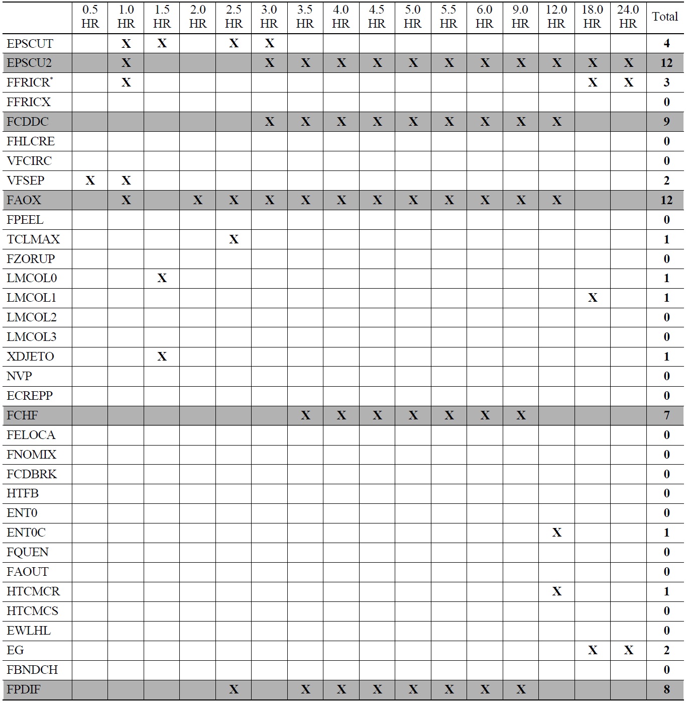
Table 4 provides a summary of the individual contributors that had a correlation greater than the threshold, indicated with an X, for the LBOP scenario.
Table 5 provides a summary of the individual contributors that had a correlation greater than the threshold,
LOOP Summary
indicated with an X, for the LOOP scenario.
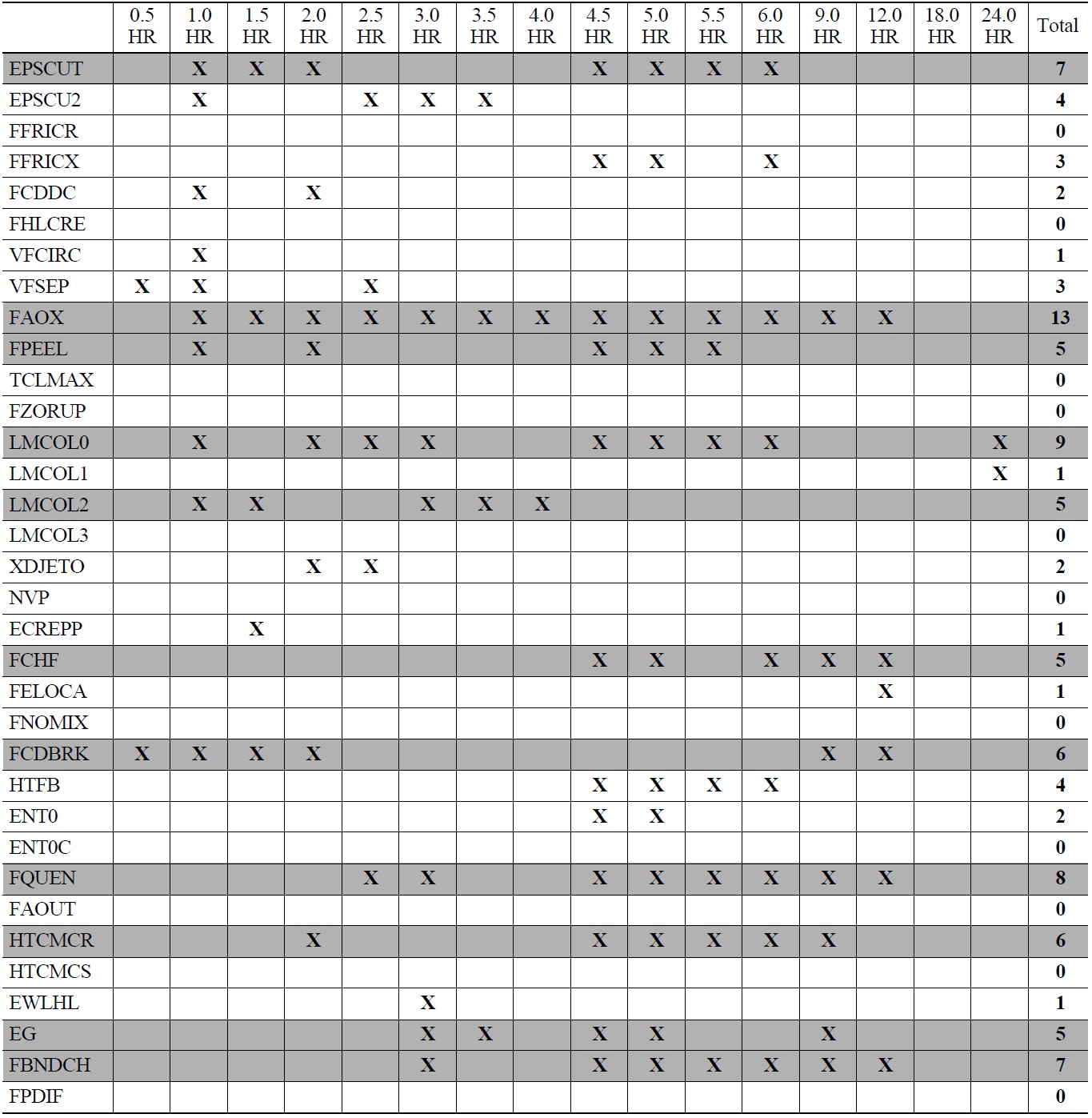
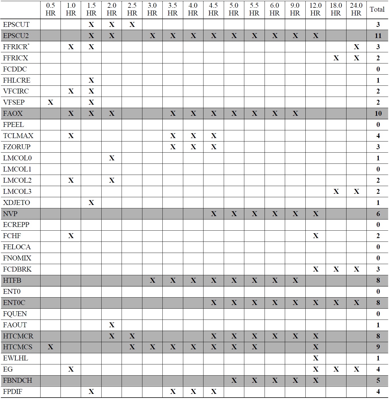
Table 6 provides a summary of the individual contributors that had a correlation greater than the threshold, indicated with an X, for the SLOCA scenario.

SLOCA Summary
Based on the results of the LBOP analysis, the following variables, appearing in more than a quarter (i.e., 5 or more) of the time intervals, have a strong correlation to hydrogen production.
EPSCU2
FCDDC
FAOX
FCHF
FPDIF
Based on the results of the LOOP analysis, the following variables, appearing in more than a quarter (i.e., 5 or more) of the time intervals, have a strong correlation to hydrogen production.
EPSCU2
FAOX
NVP
HTFB
ENT0C
HTCMCR
HTCMCS
FBNDCH
Based on the results of the SLOCA analysis, the following variables, appearing in more than a quarter (i.e., 5 or more) of the time intervals, have a strong correlation to hydrogen production.
EPSCUT
FAOX
FPEEL
LMCOL0
LMCOL2
FCHF
FCDBRK
FQUEN
HTCMCR
EG
FBNDCH
The set of parameters and their ranges (used as inputs to the uncertainty analysis) were selected based on information provided in the MAAP Zion Parameter File2 and Reference 3. The uncertainty analysis quantified the relative importance of individual contributors on how they affect Level 2 analyses. The parameters used in the analysis that did not have a strong correlation to hydrogen production are listed in Table 7 in regular text. It is recommended that the MAAP default values provided in the Zion Parameter File be used as indicated in Table 7 for these parameters. This is deemed acceptable for plants with numerous similarities to the Zion plant. The parameters used in the analysis that did have a strong correlation to hydrogen production (highlighted in Table 4, Table 5, and Table 6) are also listed in Table 7 in bold italic text. The recommendations for these values are discussed individually in the following sections.
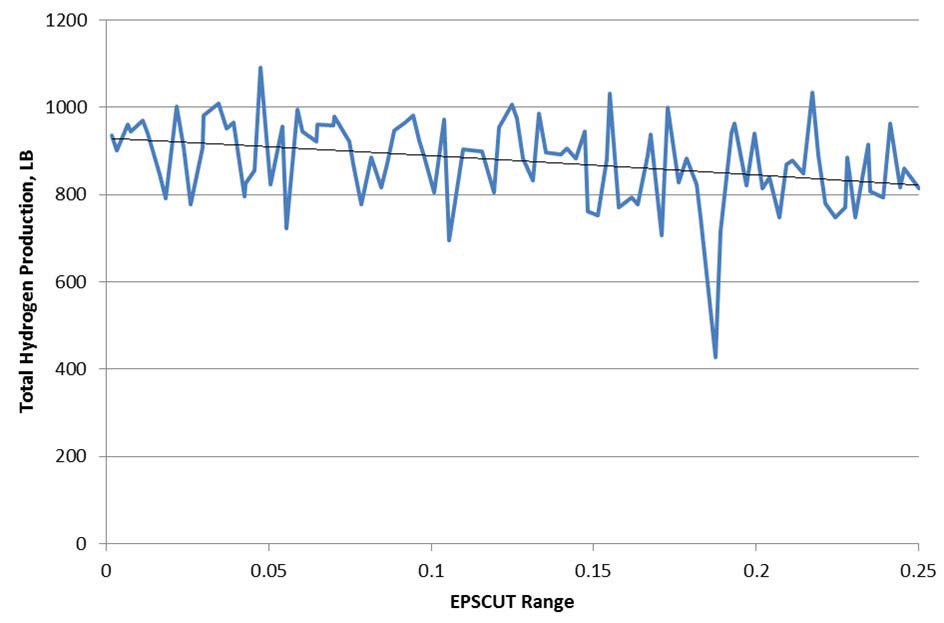
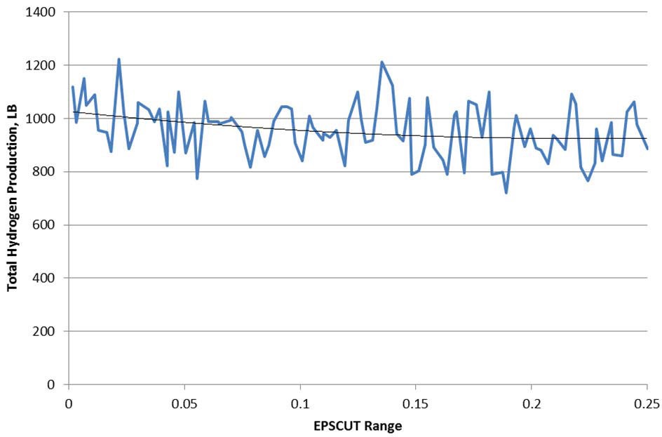
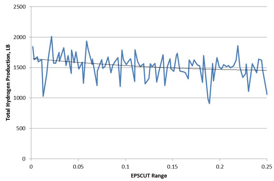
Parameter EPSCUT is the cutoff porosity below which the flow area and the hydraulic diameter of a core node are zero (the node is fully blocked). The porosity is the ratio of the free volume to the total volume within a node. This parameter effectively controls the transition from a thickened fuel pin configuration (IGTYP = 3) to a crust configuration (IGTYP = 4). This parameter can affect the amount of in-core oxidation allowed to occur since there is no oxidation in a crust configuration. The smaller the value of EPSCUT, the more material relocation is necessary for a core node to become a crust node, generally resulting in longer times for oxidation and heat transfer.
The MAAP Zion Parameter File2 indicates a range from 0.0 to 0.25. Based on the results, EPSCUT has a negative correlation to hydrogen production, meaning that as EPSCUT increases, hydrogen production decreases. A low value of EPSCUT allows for flow to continue through the damaged region for as long as possible, maximizing hydrogen production. Figure 3, Figure 4, Figure 5, and Figure 6 show the parameter EPSCUT plotted against the hydrogen production and fitted with a second order polynomial trend line at
1.0, 2.0, 5.0, and 6.0 hours respectively for the SLOCA case. The MAAP Zion Parameter File2 recommends a value of 0.1, however based on the results, a value of 0.0 would seem to be indicated. Since it is unrealistic to use a value of 0.0, a value of 0.1 is recommended providing a nominal amount of hydrogen as well as the determination of the value of EPSCU2 in the subsequent section.
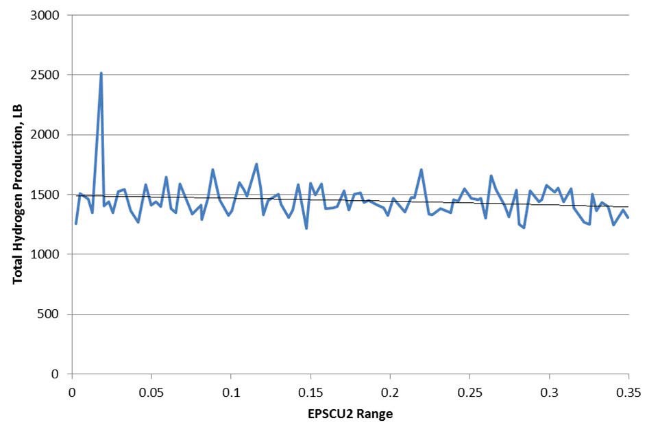
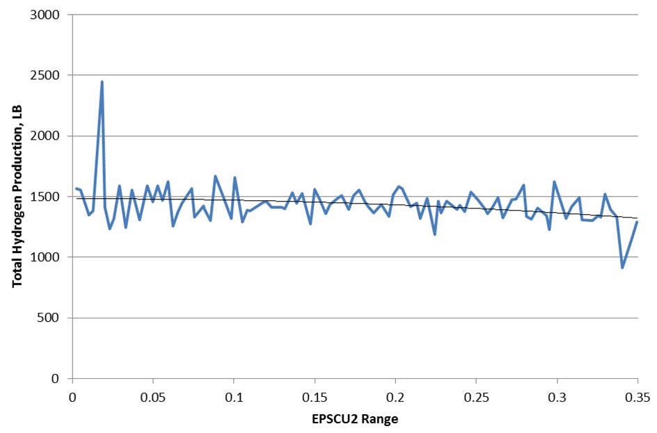
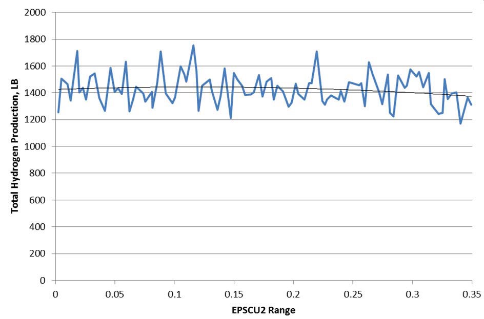
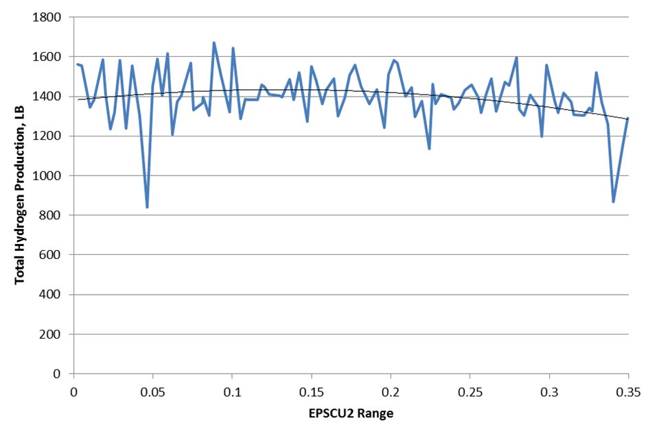
Parameter EPSCU2 is the cutoff porosity below which the flow area and the hydraulic diameter of a collapsed core node (IGTYP =2) are zero (node fully blocked). If the porosity is below this value, a blockage occurs which prevents additional core material from relocating through the blocked node. The MAAP 4 User’s Manual recommends that this parameter be less than parameter VFCRCO which was set to 0.35. The value should also be greater than the value of the model parameter EPSCUT. The smaller the value of EPSCU2, the more material relocation is necessary for a core node to become a crust node, generally resulting in longer times for oxidation and heat transfer.
The MAAP Zion Parameter File2 indicates a range from 0.001 to 0.35. Based on the results, EPSCU2 has a negative correlation to hydrogen production, meaning that as EPSCU2 increases, hydrogen production decreases. Figure 7 and Figure 8 show the parameter EPSCU2 plotted against the hydrogen production and fitted with a second order polynomial trend line at 3.0 and 12.0 hours respectively for the LBOP case. Figure 9 and Figure 10 show the parameter EPSCU2 plotted against the hydrogen production and fitted with a second order polynomial trend line at 3.0 and 12.0 hours respectively for the LOOP case. This parameter should be less than parameter VFCRCO and greater than the value of the model parameter EPSCUT. The MAAP Zion Parameter File2 recommends a value of 0.2, however based on the results, a value of 0.1 is recommended. This is approximately where hydrogen production is greatest for the LBOP and LOOP scenarios, and corresponds with the recommended value of EPSCUT provided in Section 6.1.
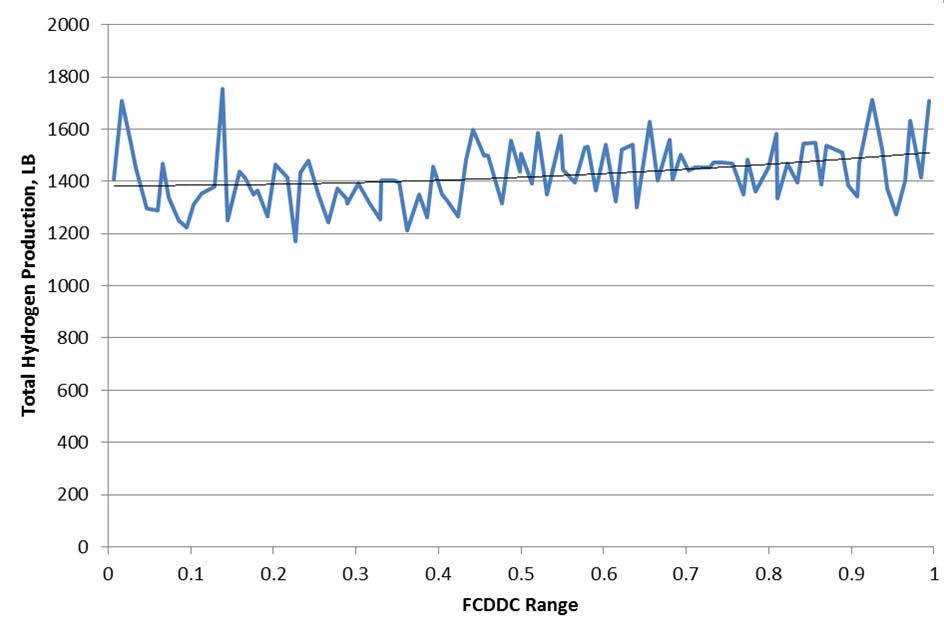
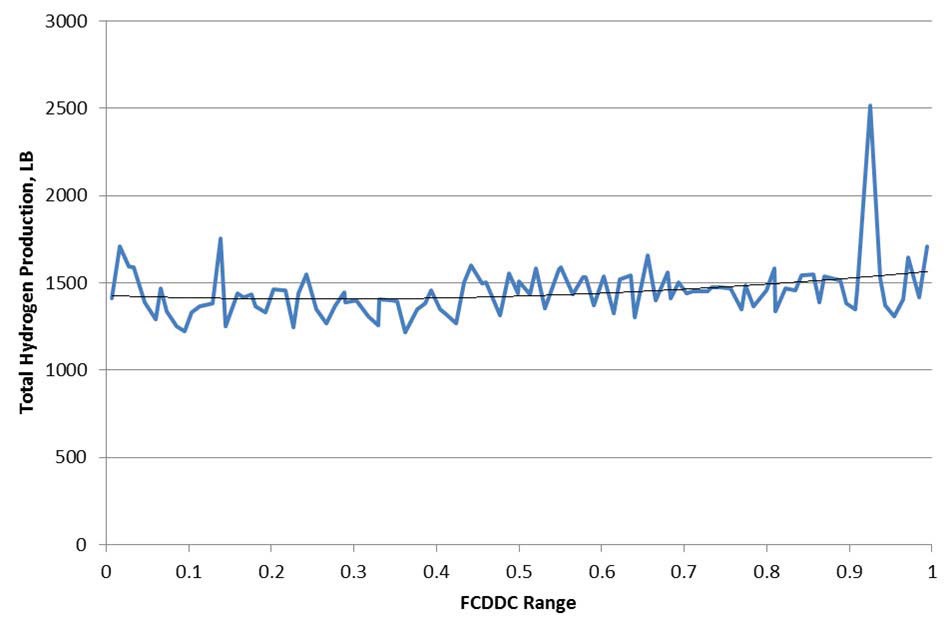
Parameter FCDDC is the maximum fraction of perfect condensation allowed for steam condensation on the free surface of water in the horizontal portion of the cold leg. A value of 0 results in no condensation being modeled. A value of 1.0 allows for perfect condensation to occur2. If a value of 1 is entered, which is the best-estimate value, the amount of condensation will be the smaller of either that computed by a simple Reynold's analogy model or that which would saturate the film of water flowing through this portion of the cold leg. FCDDC values between 0 and 1 will limit the condensation to that which will increase the enthalpy by a fraction FCDDC of the total subcooling. Depending on the injection flow rate, this parameter can affect the depressurization rate of the primary system. Users may want to use a value less than 1 when hydrogen is being generated because this reduces the potential for condensation.
The MAAP Zion Parameter File2 indicates a range from 0.0 to 1.0. Based on the results, FCDDC has a positive correlation to hydrogen production, meaning that as FCDDC increases, hydrogen production increases. Figure 11 and Figure 12 show the parameter FCDDC plotted against the hydrogen production and fitted with a second order polynomial trend line at 3.0 and 12.0 hours respectively for the LBOP case. The MAAP Zion Parameter File2 value
of 1.0 is recommended; this is approximately where hydrogen production is greatest for the LBOP scenario.
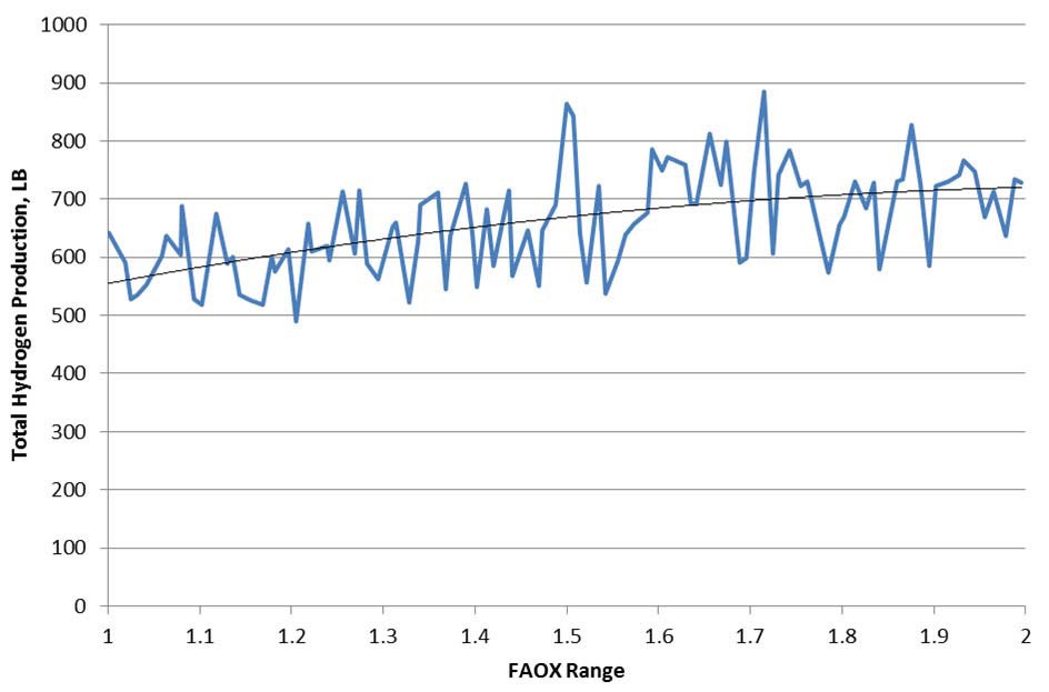
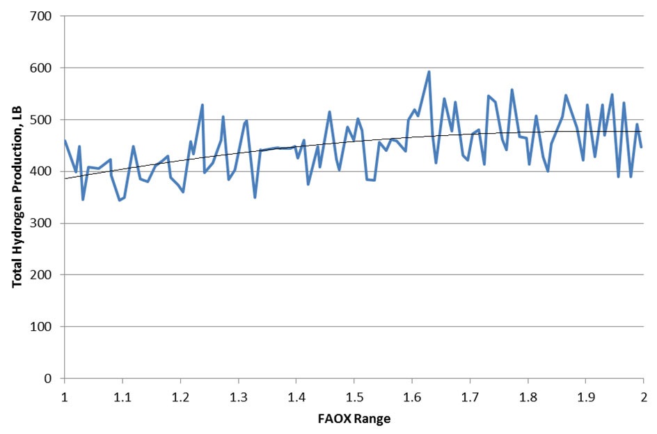
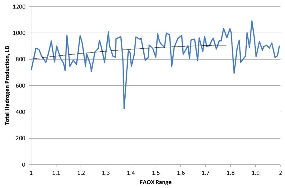
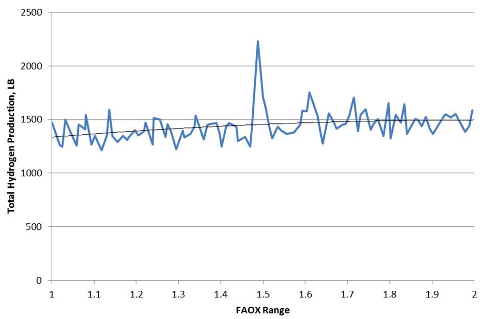
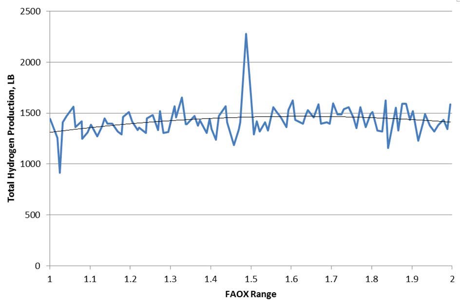
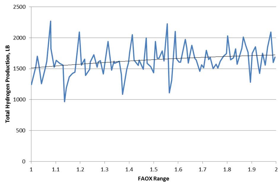
Parameter FAOX is the multiplier for the cladding outside surface area and is used in oxidation calculations to account for steam ingression after cladding rupture. Oxidation is calculated once the core is uncovered. The use of FAOX is controlled by the value of TDOOXI.
The MAAP Zion Parameter File indicates a range from 1.0 to 2.02. Based on the results, FAOX has a positive correlation to hydrogen production, meaning that as FAOX increases, hydrogen production increases. Figure 13 and Figure 14 show the parameter FAOX plotted against the hydrogen production and fitted with a second order polynomial trend line at 1.0 and 9.0 hours respectively for the LBOP case. Figure 15 and Figure 16 show the parameter FAOX plotted against the hydrogen production and fitted with a second order polynomial trend line at 1.0 and 9.0 hours respectively for the LOOP case. Figure 17 and Figure 18 show the parameter FAOX plotted against the hydrogen production and fitted with a second order polynomial trend line at 1.0 and 9.0 hours respectively for the SLOCA case. The MAAP Zion Parameter File2 value of 1.5 is recommended; this is approximately the median value.
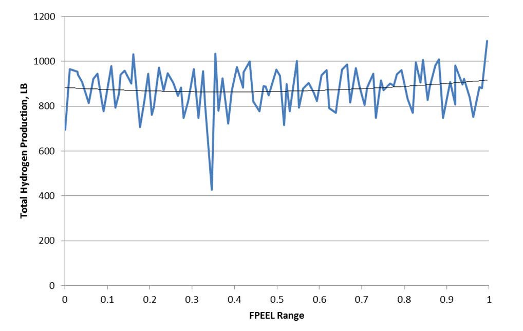
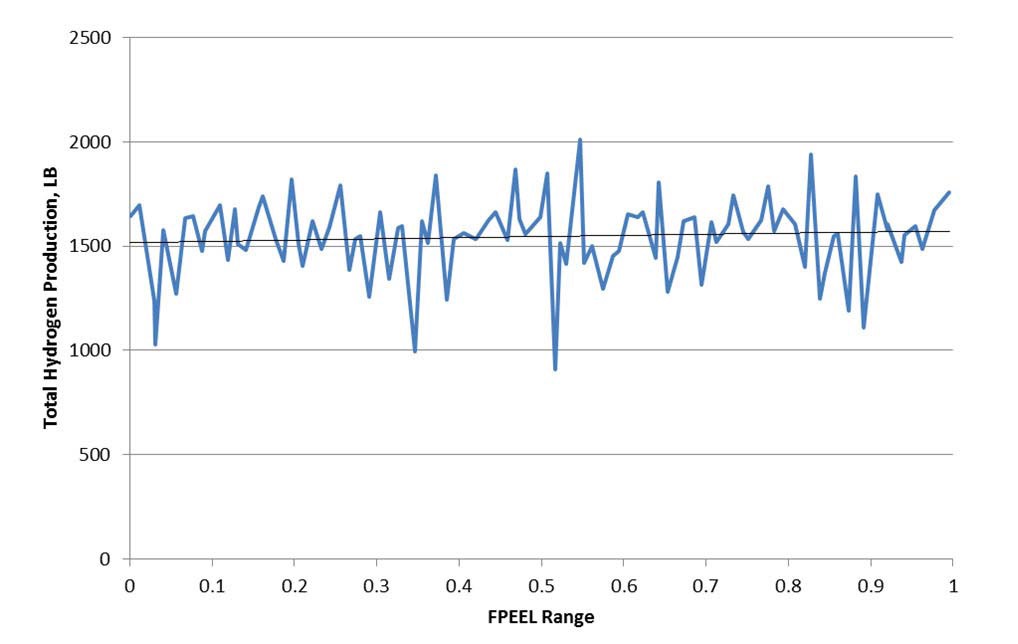
Parameter FPEEL is the fraction of the ZrO2 layer peeled off during re-flooding. According to the MAAP 4 User’s Manual2, this parameter should be set to 0.0 for the parameter file and adjusted accordingly by a local parameter change when re-flood begins.
The MAAP Zion Parameter File2 indicates a range from 0.0 to 1.0. Based on the results, FPEEL has a slight positive correlation to hydrogen production, meaning that as FPEEL increases, hydrogen production increases. Figure 19 and Figure 20 show the parameter FPEEL plotted against the hydrogen production and fitted with a second order polynomial trend line at 1.0 and 5.5 hours respectively for the SLOCA case. Based on the MAAP Zion Parameter File2 and the similarities in cladding/core material between the selected nuclear plant and the Zion plant, the MAAP Zion Parameter File2 value of 0.0 is recommended. When re-flood begins the parameter should be adjusted to 1.0 which is approximately where hydrogen production is greatest for the SLOCA scenario.
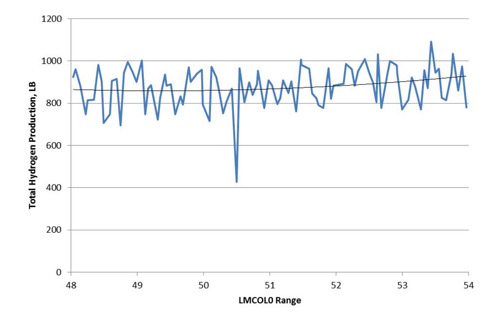
Parameter LMCOL0 is the collapse criteria parameter for a Larson-Miller functional dependence when no core node surrounding the particular core node has collapsed.
The MAAP Zion Parameter File2 indicates a range
from 48 to 54. Based on the results, LMCOL0 has a positive correlation to hydrogen production, meaning that as LMCOL0 increases, hydrogen production increases. Figure 21 shows the parameter LMCOL0 plotted against the hydrogen production and fitted with a second order polynomial trend line at 1.0 hour for the SLOCA case. Only the 1 hour time period is considered as this is an in-vessel phenomenon. The MAAP Zion Parameter File2 recommends a value of 50. However, based on the results, a value of 52.0 is recommended which is approximately the median value.
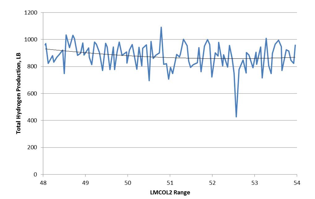
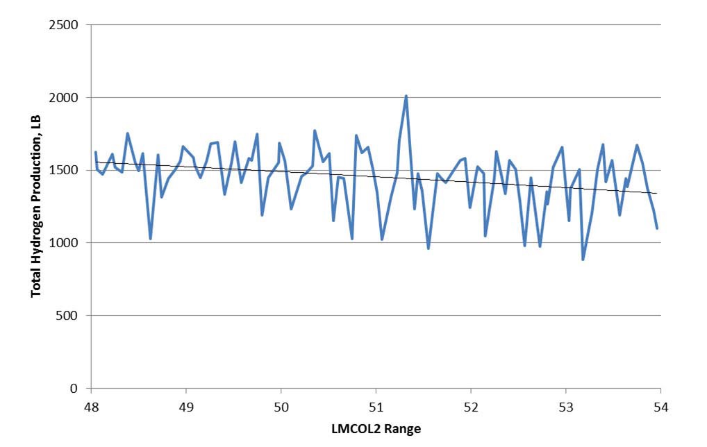
Parameter LMCOL2 is the collapse criteria parameter for a Larson-Miller functional dependence for a core node next to an empty core node.
The MAAP Zion Parameter File2 indicates a range from 48 to 54. Based on the results, LMCOL2 has a negative correlation to hydrogen production, meaning that as LMCOL2 increases, hydrogen production decreases. Figure 22 and Figure 23 show the parameter LMCOL2 plotted against the hydrogen production and fitted with a second order polynomial trend line at 1.0 and 4.0 hours respectively for the SLOCA case. Again, since this is an in-vessel phenomenon, only the early time periods were examined. The MAAP Zion Parameter File2 value of 50.0 is recommended, which is approximately the median value.
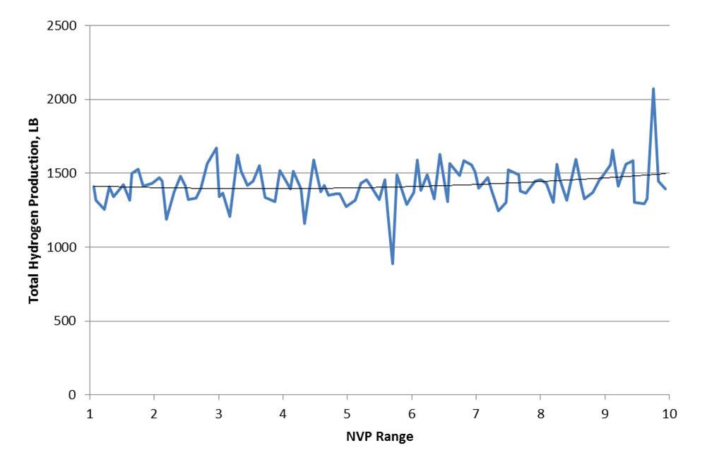
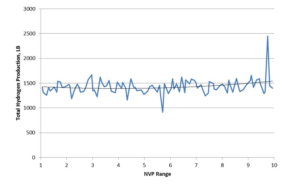
Parameter NVP is the number of corium jets emerging from the failed lower head that impact the containment floor. It determines the corium jet ablation rate of the concrete and the resulting steam and carbon dioxide generation rate. This parameter may be set equal to the number of penetrations on the failed lower head node, e.g., NPT1(i), NPT2(i), or 1 for instrument tubes, CRD tubes, or the drain line, respectively.
The MAAP Zion Parameter File2 indicates a range of 1 to 10. Based on the results, NVP has a positive correlation to hydrogen production, meaning that as NVP increases, hydrogen production increases. Figure 24 and Figure 25
show the parameter NVP plotted against the hydrogen production and fitted with a second order polynomial trend line at 4.5 and 12.0 hours respectively for the LOOP case. The distributions are nearly flat. In general, specifying a value of 1.0 for this parameter is adequate given that continuing vessel wall ablation expands the initial penetration failure radius, eventually representing more than one penetration. Therefore, the MAAP Zion Parameter File2 value of 1.0 is recommended.
Parameter FCHF is the flat plate CHF Kutateladze number. This number applies to the case of pool levitation of droplets from a heated surface in contact with an overlying water pool. The critical velocity marks the transition from a churn-turbulent pool to a fluidized bed of droplets. It is used for ex-vessel debris heat transfer only.
The MAAP Zion Parameter File2 indicates a range of 0.0036 to 0.3. Based on the results, FCHF has a positive correlation to hydrogen production, meaning that as FCHF increases, hydrogen production increases. The value of FCHF is controlled by the use of an include file for the selected nuclear plant. The value of parameter FCHF in the parameter file is irrelevant in this case and is therefore set to the recommended MAAP Zion Parameter File2 value of 0.025.
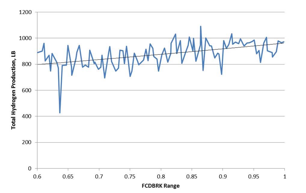
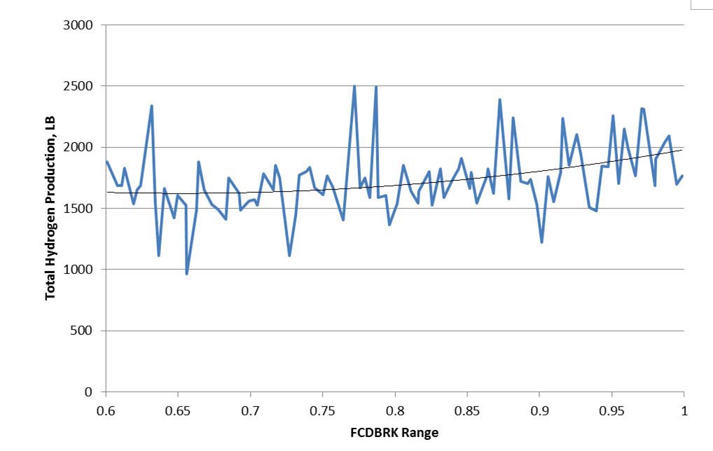
Parameter FCDBRK is the discharge coefficient for flows through primary system breaks. The calculated flows determine the primary system depressurization rate and the rate of energy deposition to the containment.
The flow is determined as follows:

where:
Abrk = LOCA break area (parameter ABB or AUB for PWRs), and
G = mass flux (a function of void fraction)
The MAAP Zion Parameter File2 indicates a range of 0.6 to 1.0. Based on the results, FCDBRK has a positive correlation to hydrogen production, meaning that as FCDBRK increases, hydrogen production increases. Figure 26 and Figure 27 show the parameter FCDBRK plotted against the hydrogen production and fitted with a second order polynomial trend line at 1.0 and 12.0 hours respectively for the SLOCA case. The value of FCDGO(1), the discharge coefficient for the first generalized opening, was set to 0.75 for the selected nuclear plant. The MAAP Zion Parameter File2 recommends a value of 0.75. However, based on the results, a value of 1.0 is recommended which is approximately where hydrogen production is greatest for the SLOCA scenario.
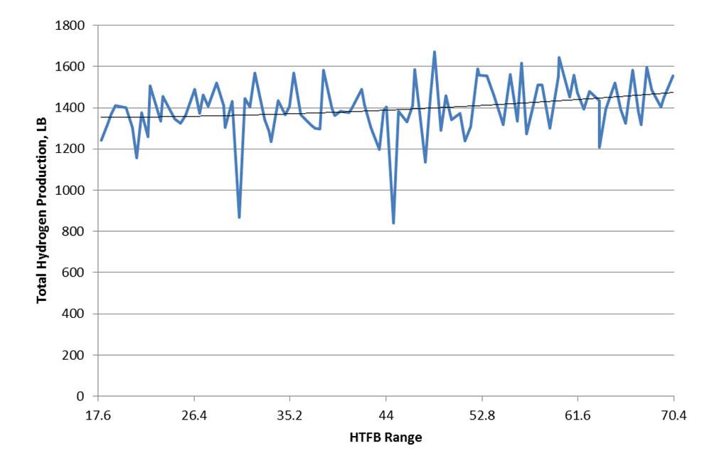
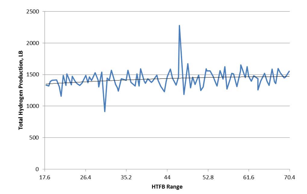
Parameter HTFB is the coefficient for film boiling heat transfer from a corium to an overlying pool.
The MAAP Zion Parameter File2 indicates a range of 17.6 to 70.4 Btu/ft2-hr-F (100 to 400 W/m2-C). Based on the results, HTFB has a positive correlation to hydrogen production, meaning that as HTFB increases, hydrogen production increases. Figure 28 and Figure 29 show the parameter HTFB plotted against the hydrogen production and fitted with a second order polynomial trend line at 3.0 and 9.0 hours respectively for the LOOP case. The MAAP Zion Parameter File2 recommends a value of 52.8 Btu/ft2-hr-F (300 W/m2-C). However, based on the results, a value of 70.4 Btu/ft2-hr-F (400 W/m2-C) is recommended which is approximately where hydrogen production is greatest for the LOOP scenario.
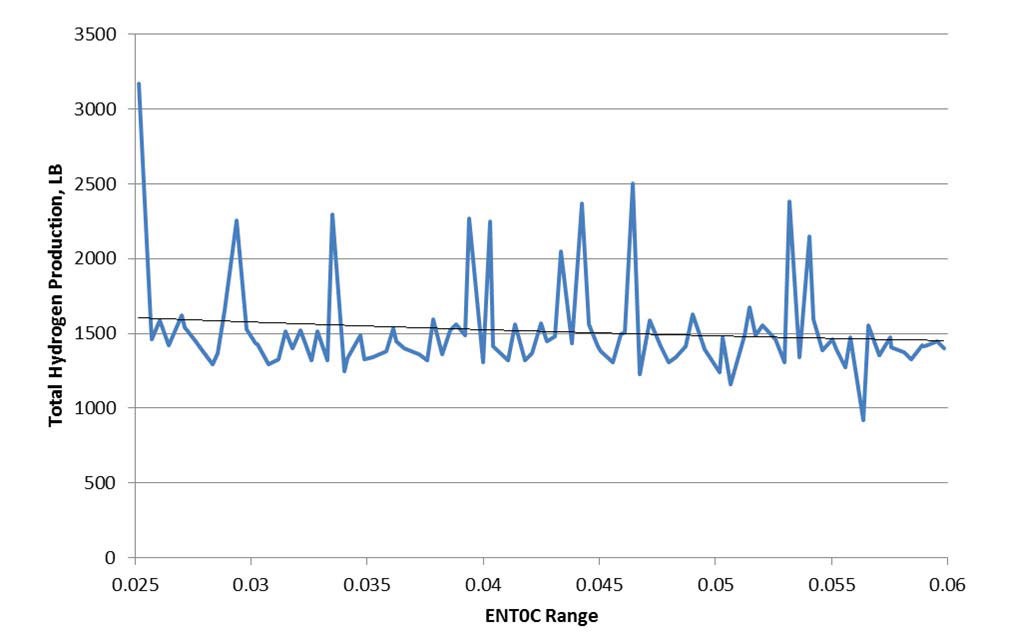
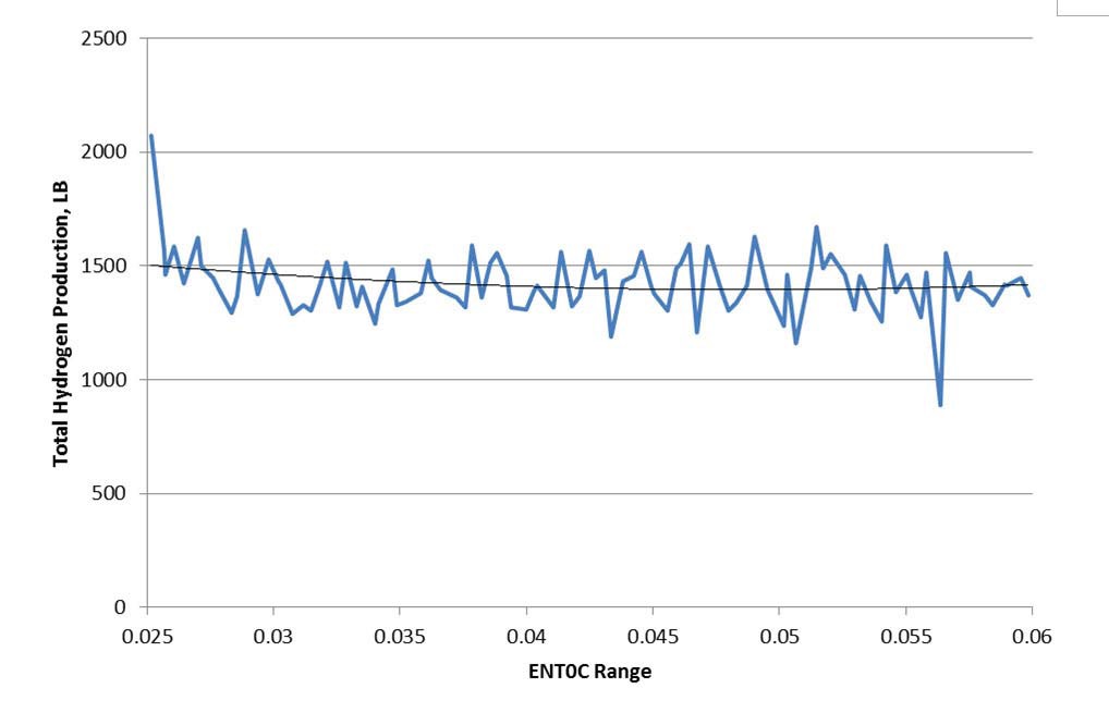
Parameter ENT0C is the jet entrainment coefficient for the Ricou-Spalding correlation which is used for debris beds within the containment. Either the input value or
one calculated using the Saito or Meignen correlations is used, depending on the value of control parameter IENT0. The input or calculated value is then used to calculate the entrainment of a corium jet entering a water pool in the containment. ENT0C is used to determine how large a fraction of the molten jet from the lower plenum will be entrained and become particulated as it pours through the water pool in the containment. The state of the debris bed in containment, mostly particulated or mostly molten (continuous bed), will determine whether the debris bed is quenchable or not. Increasing ENT0C increases the amount of entrainment.
The MAAP Zion Parameter File2 indicates a range of 0.025 to 0.06. Based on the results, ENT0C has a negative correlation to hydrogen production, meaning that as ENT0C increases, hydrogen production decreases. Figure 30 and Figure 31 show the parameter ENT0C plotted against the hydrogen production and fitted with a second order polynomial trend line at 4.5 and 24.0 hours respectively for the LOOP case. The MAAP Zion Parameter File2 recommends a value of 0.045. However, based on the results, a value of 0.025 is recommended which is approximately where hydrogen production is greatest for the LOOP scenario and will produce particulate debris particles with a size of 2.5
millimeters, maximizing the surface area for potential oxidation.
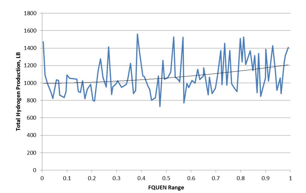
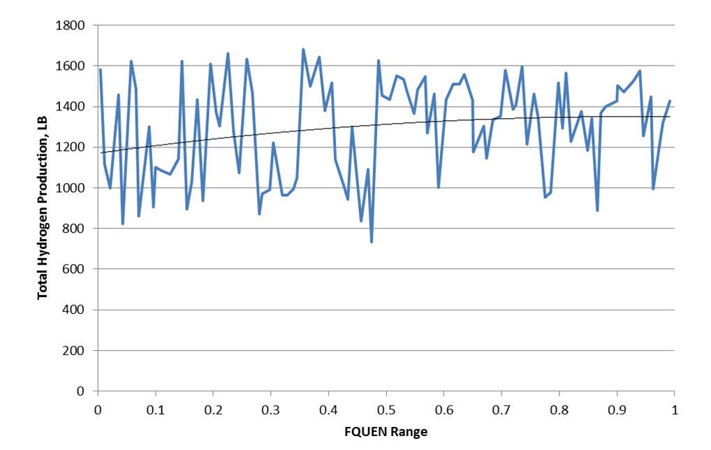
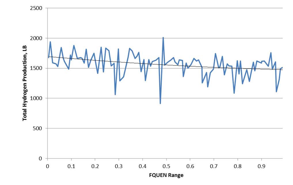
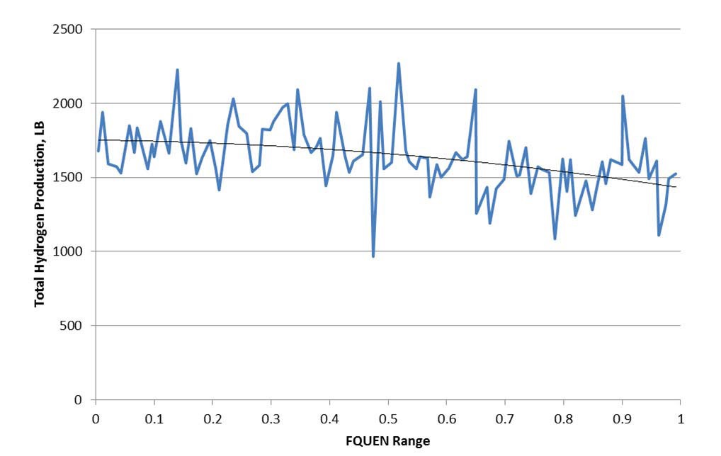
Parameter FQUEN is the multiplier to the flat plate CHF for lower head debris bed quenching by overlying water. A value of 0 means the metal layer is impermeable to water. This parameter is used to investigate the effects of water ingression into the debris bed in the RPV lower plenum.
The MAAP Zion Parameter File2 indicates a range of 0.0 to 1.0. Based on the results, FQUEN has a positive correlation to hydrogen production early in the SLOCA scenario, meaning that as FQUEN increases, hydrogen production increases,. FQUEN has a negative correlation to hydrogen production later in the SLOCA scenario, meaning that as FQUEN increases, hydrogen production decreases. Figure 32, Figure 33, Figure 34, and Figure 35 show the parameter FQUEN plotted against the hydrogen production and fitted with a second order polynomial trend line at 2.5, 3.0, 6.0, and 9.0 hours respectively for the SLOCA case. The MAAP Zion Parameter File2 recommends a value of 0.2. Based on the results, this parameter behaves differently for the two periods. The positive
correlation to hydrogen production early in the scenario is due to in-vessel phenomena and the negative correlation later is due to ex-vessel phenomena, meaning the early oxidation results in less external hydrogen production. Therefore, the MAAP Zion Parameter File2 value of 0.2 is recommended.
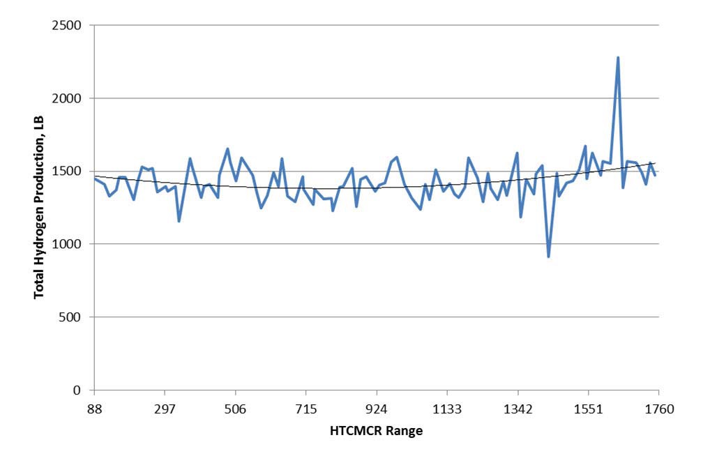
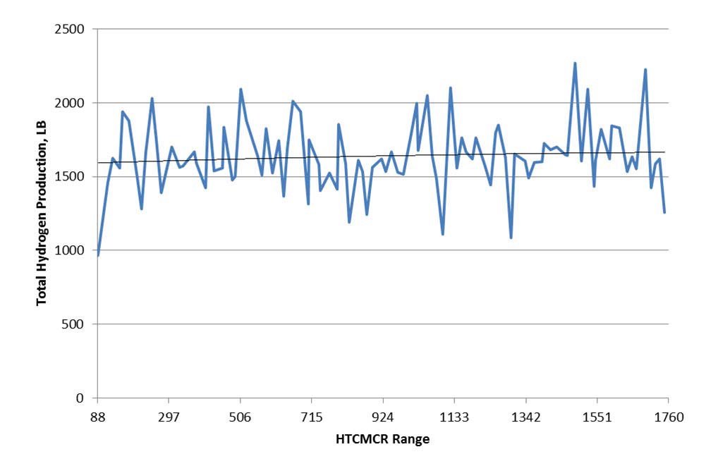
Parameter HTCMCR is the nominal downward heat transfer coefficient for convective heat transfer from molten corium to the lower crust for corium-concrete interaction calculations. It is used to calculate the actual heat transfer coefficient, HTD, via the expression:

where FSOL is the corium solid fraction and CDU is the exponent used to calculate the downward and sideward heat transfer coefficients for convective heat transfer from molten corium to the lower and side crusts, respectively, for corium-concrete interaction calculations.
The meaning of this parameter was slightly modified for MAAP 4.0.7. The new options are as follows:
> 0: use parameter in conventional manner
< 0: exercise the option of specifying corium poolspecific parameter ? See parameter HTCMFLR (IC) in the MAAP 4 User’s Manual2
The MAAP Zion Parameter File2 indicates a range of 88 to 1760 Btu/ft2-hr-F (500 to 10000 W/m2-C). Based on the results, HTCMCR has a positive correlation to hydrogen production in the LOOP scenario and in the SLOCA scenario, meaning that as HTCMCR increases, hydrogen production increases. Figure 36 and Figure 37 show the parameter HTCMCR plotted against the hydrogen production and fitted with a second order polynomial trend line at 9.0 hours for the LOOP and SLOCA cases respectively. Heat transfer coefficients tend to be self-correcting as shown in the figures. Therefore, the MAAP Zion Parameter File2 value of 616 Btu/ft2-hr-F (3500 W/m2-C) is recommended.
Parameter HTCMCS is the nominal sideward heat transfer coefficient for convective heat transfer from molten to the side crust for corium-concrete interaction calculations. It is used to calculate the actual heat transfer coefficient, HTS, via the expression shown below

where FSOL is the corium solid fraction and CDU is the exponent used to calculate the downward and sideward heat transfer coefficients for convective heat transfer from molten corium to the lower and side crusts, respectively, for corium-concrete interaction calculations.
The meaning of this parameter was slightly modified for MAAP 4.0.7. The new options are as follows:
> 0: use parameter in conventional manner
< 0: exercise the option of specifying corium poolspecific parameter ? See parameter HTCMSID(IC) in the MAAP 4 User’s Manual2
The MAAP Zion Parameter File2 indicates a range of 88 to 1760 Btu/ft2-hr-F (500 to 10000 W/m2-C). Based on the results, HTCMCS has a positive correlation to hydrogen production in the LOOP scenario, meaning that as HTCMCS increases, hydrogen production increases. Figure 38 shows the parameter HTCMCS plotted against the hydrogen production and fitted with a second order polynomial trend line at 12.0 hours for the LOOP case. Heat transfer coefficients tend to be self-correcting. Therefore, the MAAP Zion Parameter File2 value of 528 Btu/ft2-hr-F (3500 W/m2-C) is considered to be adequate.
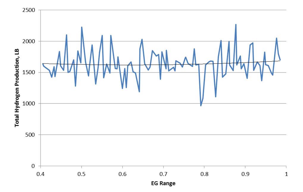
Parameter EG is the emissivity of gas. It is essentially the emissivity of steam because the emissivity of the other gases is generally small.
The MAAP Zion Parameter File2 indicates a range of 0.4 to 0.99. Based on the results, EG has a positive correlation
to hydrogen production in the SLOCA scenario, meaning that as EG increases, hydrogen production increases. Figure 39 and Figure 40 show the parameter EG plotted against the hydrogen production and fitted with a second order polynomial trend line at 3.0 and 9.0 hours respectively for the SLOCA case. Table 4-5 of EPRI Report 102023621 recommends the default value should be used. The MAAP Zion Parameter File2 recommends a value of 0.65. However, based on the results, a value of 0.99 is recommended which is approximately where hydrogen production is greatest for the SLOCA scenario.
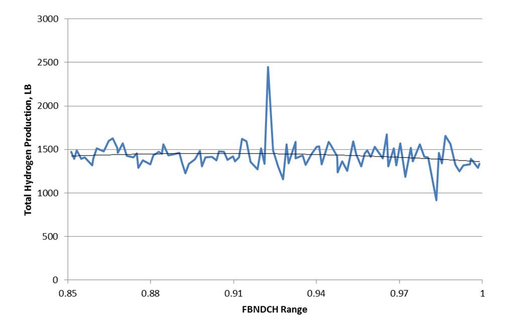
Parameter FBNDCH is the hydrogen jet burning factor during high pressure melt ejection/ direct containment heating (HPME/DCH). The burning of hydrogen jets during HPME/DCH is controlled by this parameter in conjunction with the DCH flag set by DCH1/DCH2. FBNDCH is used as a multiplier to the normal jet flow rate to account for turbulent jet entrainment.
The MAAP Zion Parameter File2 indicates a range of 0.85 to 1.0. Based on the results, FBNDCH has a negative correlation to hydrogen production in the LOOP scenario, meaning that as FBNDCH increases, hydrogen production decreases. FBNDCH has a positive correlation to hydrogen production in the SLOCA scenario, meaning that as FBNDCH increases, hydrogen production increases. As this parameter is directed towards HPME events, the higher pressure scenario (LOOP) is chosen to be the more representative scenario for this parameter as opposed to the lower pressure event (SLOCA). Figure 41 and Figure 42 show the parameter FBNDCH plotted against the hydrogen
production and fitted with a second order polynomial trend line at 5.0 and 12.0 hours respectively for the LOOP case. The MAAP Zion Parameter File2 recommends a value of 1.0. However, based on the results, a value of 0.90 is recommended which is approximately where hydrogen production is greatest for the LOOP scenario.
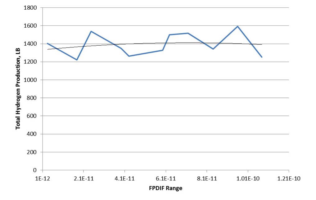
Parameter FPDIF is the diffusivity of fission products migrating through the molten material for the DCH1 model. It is used to calculate the fission product release from the particulated debris.
Note: The units of diffusivity are not converted in the code. Hence, the value for FPDIF should be in SI units (m2/s) for a parameter file that is in British units.
The MAAP Zion Parameter File2 indicates a range of 0.1×10⁻¹² to 0.1×10-09 m2/s (see footnote in Table 2). The range inadvertently used in this analysis is 1.0×10⁻¹² to 1.0×10-09 m2/s. While the values are different, the span of the range still covers 3 orders of magnitude, which should be sufficient in determining correlation. Based on the results, FPDIF has a positive correlation to hydrogen production in the LBOP scenario, meaning that as FPDIF increases, hydrogen production increases. Figure 43 and Figure 44 show the parameter FPDIF plotted against the
[Table 7.] Parameters Examined for Level 2 Statistical Analysis
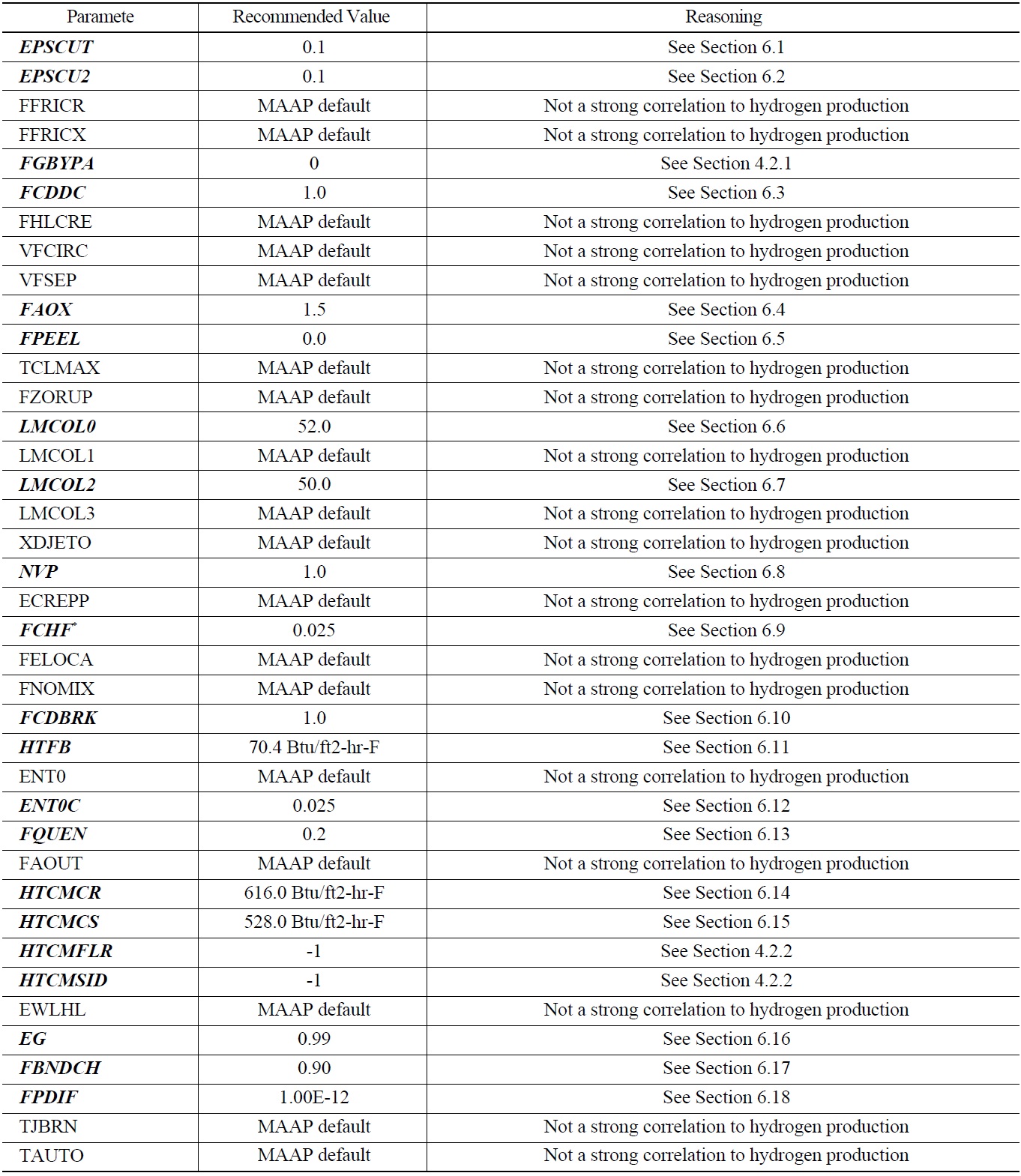
Parameters Examined for Level 2 Statistical Analysis
hydrogen production and fitted with a second order polynomial trend line at 9.0 and 2.5 hours respectively for the LBOP case. The range used in the plots is 1.0×10⁻¹² to 1.0×10⁻¹⁰ m2/s to coincide with the actual range from the parameter file. As this parameter is associated with early DCH events, the effect of this parameter was not expected to change after the initial major relocation of the core. This is illustrated by Figure 44 which shows nearly identical results to those at 9.0 hours. The MAAP Zion Parameter File2 recommends a value of 1.0×10⁻¹¹ m2/s. However, based on the results, a value of 8.0×10⁻¹¹ m2/s is recommended which is approximately where hydrogen production is greatest for the LBOP scenario.
This paper has demonstrated that by using standard statistical methods, the key parameters affecting a desired dependent phenomenon (hydrogen for the case presented) can be identified along with an appropriate value to either minimize or maximize the quantity.
Pr{|hRS|2 ≥ g(ρ)} Pr{|hDS|2 + |hDR|2 < g(ρ) } + Pr{|hRS|2 < g(ρ)}Pr{|hDS |2≥g(ρ)},
where
whose high SNR behavior is readily shown to be
due to the fact that