The scale invariant feature transform (SIFT) is an effective algorithm used in object recognition, panorama stitching, and image matching. However, due to its complexity, real-time processing is difficult to achieve with current software approaches. The increasing availability of parallel computers makes parallelizing these tasks an attractive approach. This paper proposes a novel parallel approach for SIFT algorithm implementation using a block filtering technique in a Gaussian convolution process on the SIMD Pixel Processor. This implementation fully exposes the available parallelism of the SIFT algorithm process and exploits the processing and input/output capabilities of the processor, which results in a system that can perform real-time image and video compression. We apply this implementation to images and measure the effectiveness of such an approach. Experimental simulation results indicate that the proposed method is capable of real-time applications, and the result of our parallel approach is outstanding in terms of the processing performance.
Nowadays, image matching is used for solving many problems in the field of computer vision, such as object or scene recognition, three-dimensional (3D) structure from multiple images, stereo correspondence, and motion tracking. In recent years, an approach has been proposed to generate a set of salient image features. This approach is called the scale invariant feature transform (SIFT); it transforms image data into scale-invariant coordinates with respect to local features. SIFT is a complex algorithm, and when used in multimedia applications, it is necessary to find a scheme to implement the algorithm in real-time.
In the previous approaches, the SIFT algorithm was implemented in both software and hardware. Due to the complexity of the SIFT algorithm, the software implementation cannot be applied in real-time applications. Therefore, recent research has mainly focused on the implementation and acceleration of the SIFT algorithm in hardware. Some approaches use the graphic processing unit (GPU) for the SIFT algorithm implementation. Sinha et al. [1] applied SIFT on a GPU; however, because of the hardware and OpenGL limitations, some data transfers were required between the GPU and the central processing unit (CPU), resulting in an increase in the data transmission time. As a result, their implementation can process a 640 × 480 video at the speed of 10 frames per second (FPS). Another approach is the SIFT implementation on multi-core systems proposed by Zhang et al. [2]. This approach takes advantage of the computing power of multi-core processors like dualsocket and quad-core systems. In their experiments, Zhang et al. [2] observed that the processing speed achieves an average of 45 FPS for a 640 × 480 video. However, more fine-grain-level parallelization must be conducted to reduce the load imbalance and achieve maximum performance with this approach in future large-scale multi-core systems.
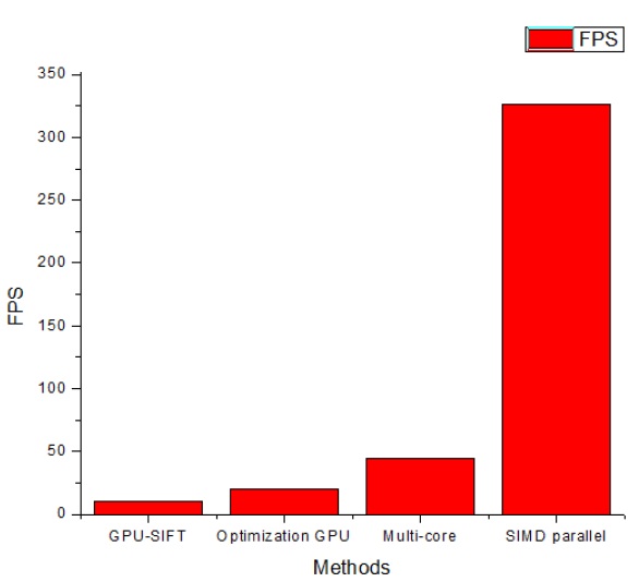
The single instruction multiple data (SIMD) pixel processor array, which has not previously been proposed for SIFT algorithm implementation purposes, is used in our implementation to address the major draw-backs of previous research. To adapt the SIFT algorithm implementation to the data parallel architecture, we propose a parallelization SIFT algorithm approach called the P-SIFT algorithm. In the P-SIFT implementation, block filtering [3] is used for calculating the Gaussian filter to improve the performance. The SIMD pixel processor can exploit the benefits of integrating optoelectronic devices into a high-performance digital processing system and fully exposes the available parallelism calculation of the P-SIFT algorithm. We have evaluated the impact of our parallel approach based on the processing performance. In the experiment detail section, we report that the processing speed is 326 FPS in the case of a 640 × 480 video. Compared with the existing hardwarebased SIFT implementations [1,2,4], our approach achieves a speed that is around 7 to 30 times faster. Further, because of the fine-grain characteristic of the SIMD pixel processor, we show that the load imbalance of our implementation is reduced.
The rest of this paper is organized as follows: In Section II, we briefly describe the related research. In Section III, a novel P-SIFT that uses block filtering is proposed. Section IV discusses the SIMD pixel processor system and the lowmemory SIMD architecture. Section V describes in detail how the proposed algorithm has been adapted to fully exploit the unique capability of the SIMD processor system. Strong proposals for the performance of the system and the experimental results are presented in Section VI. Section VII concludes this paper with a presentation of the simulation results.
SIFT is perhaps the most popular invariant local feature detector at present and has been applied successfully on many occasions, such as object recognition, image match and registration, structure from motion and 3D reconstruction, visual simultaneous localization and mapping and image panorama.
Nevertheless, the complexity of the SIFT algorithm results in a very high time consumption. Because of the high popularity of SIFT, it is no surprise that several variants and extensions of SIFT have been proposed. For example, Ke and Sukthankar [5] proposed the PCA-SIFT that applies principal component analysis (PCA) to the normalized gradient patch. The Gradient location and orientation histogram (GLOH) [6] changes the SIFT’s location grid and uses PCA to reduce the size of SIFT. The primary focus of these extensions is to gain improved performance.
An approach called Harris-SIFT [7] removes many indistinctive candidates before generating descriptors, thus saving excessive computations. Harris-SIFT reduces both the feature number and the database size, or in other words, cuts down the feature matching time. However, as provided, the results of the Harris-SIFT method are not sufficiently fast to be implemented in real time.
In the fast approximated SIFT, Grabner et al. [8] proposed a modified SIFT method for recognition purposes. The authors sped up the SIFT computation by using approximations (mainly employing integral images) in both the difference of Gaussian (DoG) detector and the SIFT descriptors. Their method can reduce the SIFT computation time by a factor of eight as compared to the binaries SIFT proposed by Lowe [9]. However, the loss in matching performance is a major drawback of this approach.
In the above approaches, the authors attempted to improve the performance of the SIFT algorithm by the modification of SIFT. However, for real-time implementation purposes, some hardware-based approaches have been proposed in recent years. Sinha et al. [1] presented GPU-SIFT, a GPUbased implementation for the SIFT feature extraction algorithm. The GPU-SIFT has been implemented using the OpenGL graphics library and the Cg shading language and tested on modern graphics hardware platforms. Their implementation can process a 640 × 480 video at 10 FPS. The weakness of this approach can be attributed to the hardware and OpenGL limitations. Some data transfers are required between the GPU and the CPU and thus take time for data transition. Another approach that also used a GPU was developed by Heymann et al. [4]. In this research, the authors showed how a feature extraction algorithm can be adapted to make use of modern graphics hardware. Their experiment used NVIDIA Quadro FX 3400 GPU with 256- MB video RAM. As a result, the SIFT algorithm can be applied to image sequences with 640 × 480 pixels at 20 FPS. Further, recently, with the development of embedded technology, a new implementation of SIFT on a multi-core processor has been proposed by Zhang et al. [2]. In their approach, the SIFT algorithm is implemented on multi-core processors like dual socket and quad-core systems. The obtained result is an average of 45 FPS for a 640 × 480 video.
III. P-SIFT ALGORITHM USING BLOCK FILTERING
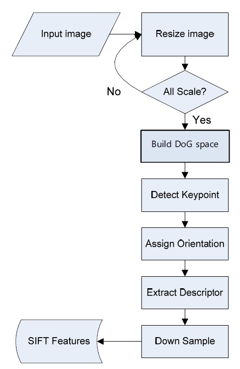
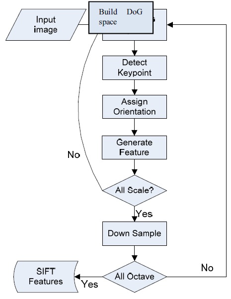
The SIFT algorithm [10] combines a scale invariant region detector and a descriptor based on the gradient distribution in the detected regions. The descriptor is presented by a 3D histogram of gradient locations and orientations. These descriptors (local features) are very distinctive and invariant for image scaling or rotation. The flowchart of the SIFT algorithm is shown in Fig. 1. In this flowchart, there are four major steps [9]: DoG space building, keypoint detection and localization, orientation assignment, and the keypoint descriptor. DoG space building: scale-space extrema detection stage of the filtering attempts to equate different viewpoints that are the projections of a specific 3D object point. They are then examined in further detail. The identification of candidate locations can be efficiently achieved using the continuous “scale space” function, which is based on the Gaussian function. The scale space is defined by the following function:

SIFT is one such technique that locates the scale-space extrema from the Gaussian image differences

In Eqs. (1) and (2), * denotes the convolution operator,
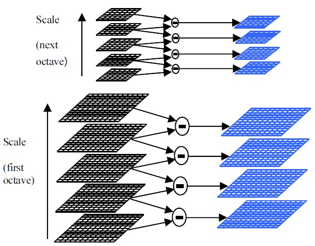
The construction of the DoG space is illustrated in Fig. 2. The initial image is repeatedly convolved with Gaussians to generate the set of scale-space images. The adjacent Gaussian images are subtracted to produce the DoG images as shown on the right of the figure.
The Gaussian image is down-sampled by a factor of 2 after each octave, and the process repeated. The convolved images are grouped by octave, and the number of DoG per octave is fixed. Keypoint detection and localization: To detect the local maxima or minima of
The keypoint localization stage attempts to eliminate these points from the list of keypoints that have low contrast (and are therefore sensitive to noise) or have poorly localized edges. This is achieved by calculating the Laplacian value for each keypoint found in the previous stage. The location of the extrema, z, can be expressed as follows:
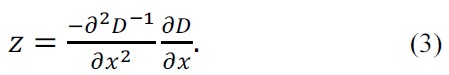
If the function value at z is below a threshold value, then this point is discarded. This removes the extrema that have a low contrast.
Edge extrema that have large principle curvatures but small curvatures in the perpendicular direction are eliminated. Using the 2 × 2 Hessian matrix
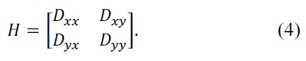
The elimination criteria can be constructed as follows:
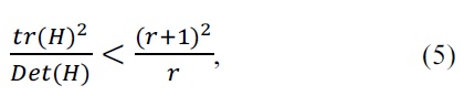
where
If this inequality is true, the keypoint is rejected.
The orientation assignment stage in Fig. 1 aims to assign a consistent orientation to the keypoints based on the local image properties. The keypoint descriptor is represented relative to this orientation because it is invariant to the rotational movements of the keypoints. The approach taken to find an orientation uses the keypoint scale to select the Gaussian smoothed image
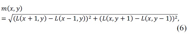
Then, we form an orientation histogram from the gradient orientations of the sample points, and locate the highest peak in the histogram. We use this peak and any other local peak within 80% of the height of this peak to create a keypoint with the orientation
The local gradient data, used above, are also used for creating keypoint descriptors. The gradient information is rotated to line up with the orientation of the keypoint and then weighted by a Gaussian kernel with a variance of the keypoint scale multiplied by 1.5. These data are then used for creating a set of histograms over a window centered on the keypoint.
Keypoint descriptors typically use a set of 16 histograms, which are aligned in a 4 × 4 grid, each with 8 orientation bins, one for each of the main compass directions and one for each of the mid-points of these directions. These result in a feature vector containing 128 elements.
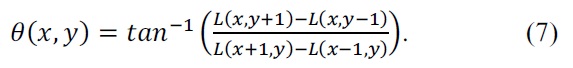
The distribution of computation time (measured in seconds) for each stage in the SIFT algorithm
These resulting vectors are known as SIFT keys and are used in the nearest-neighbors approach to identify possible objects in an image. Collections of keys that agree on a possible model are identified. When three or more keys agree on the model parameters, the model is evident in the image.
We processed images using the C++ code developed by Lowe [9] and then measured the performance. The obtained results (Table 1) show that most of the calculations are implemented in the first stage: DoG space building. In this step, many calculations are repeatedly processed. Based on this characteristic, we propose a parallel approach for the SIFT algorithm called P-SIFT. The proposed algorithm can take advantage of parallelism. The P-SIFT will be described in detail in subsection III-B. In subsection III-A, we present a new method to calculate the Gaussian filter called block filtering.
>
A. Block Filtering Technique
In the SIFT algorithm, the Gaussian filter is used many times during the SIFT feature determination. For calculation time reduction purposes, we propose a new method to implement the Gaussian convolution. In the proposed method, we use a 4 × 4 block to implement the Gaussian filter.
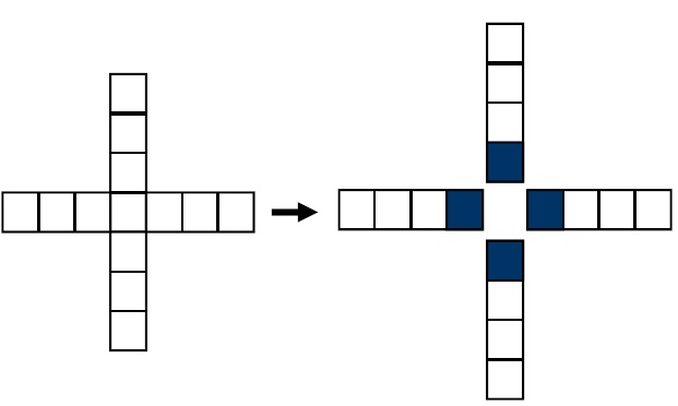
For example, we divide the image into sub-blocks. The size of these blocks is 4 × 4 pixels. Then, we apply a half kernel to the block; in this case, it is an array with four elements. In Fig. 3, we explain the “half kernel” definition. Because of the symmetric characteristic of the Gaussian kernel, we divide the Gaussian kernel into four “half kernels.”
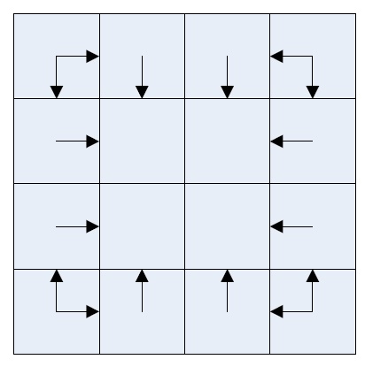
Fig. 4 demonstrates how these blocks are applied to the image. After loading each 4 × 4 block of the input image. These “half kernels” are applied in four directions (left, right, top, and bottom) to the 4 × 4 block.
The proposed Gaussian filter implementation using the block filtering technique includes the following four steps:
1. Load 4 × 4 pixels of image.
2. Load kernel values.
3. Compute convolution (left, right, top, and bottom). Left, Right: reverse multiplication Top: Matrix transpose Bottom: Matrix transpose and then reverse multiplication
4. By repeating all image data, we will obtain the output image.
Our previous research [10] indicated that by using the block filtering for a Gaussian filter, we can reduce the calculation time by half.
As evident from the flowchart of the original SIFT algorithm (Fig. 5), each keypoint will be assigned an orientation and generate a descriptor just after detecting the keypoints for one scale. In this case, if we only detect a few keypoints in the later iterations of the octaves and the scales, there may be very few keypoints for the next computational step. This implies that the load imbalance will occur in the “Assign Orientation” and “Extract Descriptor” steps for each keypoint.
Moreover, the number of keypoints detected from each scale is decreased gradually when the image is downsampled. Because of this, load balance can be a serious issue in the later stages.
Further, the original SIFT algorithm is implemented in a straightforward manner. In this case, the speed of SIFT is quite poor. In the straight implementation, SIFT feature detection is repeated for each image in the scale space. Therefore, we have to repeat the same operation many times. To take advantage of the parallelization characteristic, we propose a parallel approach to implement the SIFT algorithm.
In our approach, we propose a parallel SIFT algorithm (PSIFT) to adapt to the SIMD processor architecture. The flowchart of P-SIFT is illustrated in Fig. 5. The first step is to resize the input image into many images in the scale space. In our implementation, the number of images in the scale space is changed from 2 to 4. Then, we consider all images in the scale space and apply the SIFT feature detection process simultaneously.
IV. SIMD PROCESSOR ARRAY ARCHITECTURE
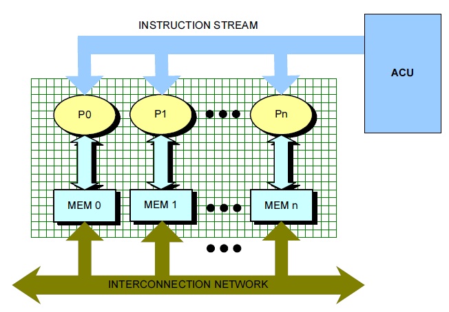
The SIMD pixel processor system [11] exploits the benefits of integrating optoelectronic devices into a highperformance digital processing system. In this system, an array of thin-film detectors is integrated on top of and electrically interfaced with digital SIMD processing elements. The general architecture of a SIMD system is depicted in Fig. 6. The program is stored in the array control unit, and each instruction is broadcast to every node of the system in a lockstep fashion (i.e., via a single instruction stream). Each node, in turn, executes the received instructions on its local data (multiple data stream), while exchanging data with other nodes through the interconnection network.
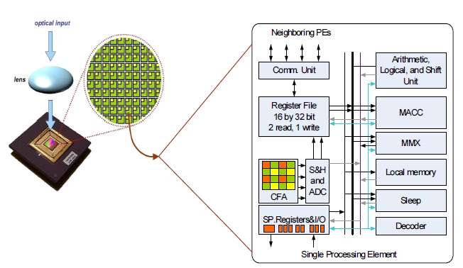
Each SIMD processor node is interconnected to its four neighbors through a mesh network closed as a torus. Thus, the opposite rows (or columns) of the mesh are connected to each other, enabling more powerful communication schemes than those available with a standard North-East- West-South (NEWS) network. The microarchitecture of an SIMD processing element (PE) is shown in Fig. 7, along with the interconnection network. The 16-bit data path includes an adder-subtractor, barrel shifter, and multiplyaccumulator unit. Each PE also includes 64 words of local memory.
Further, each SIMD processor node interfaces with a small array of thin film detectors, which is a subset of the focal plane array. The instruction set architecture allows a single node to address up to 16 × 16 arrays of detectors. Each processor incorporates eight-bit sigma-delta analog to digital converters to convert light intensities, incident on the detectors, into digital values. The SAMPLE instruction simultaneously samples all detectors values and makes them available for further processing. The SIMD execution model allows the entire image projected on many nodes to be sampled in a single cycle.
This monolithic integration is the key feature of the SIMD pixel processor system, providing extremely compact, high-frame-rate focal plane processing.
V. SIMD PROCESSOR ARRAY ARCHITECTURE
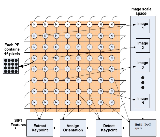
To execute the P-SIFT algorithm, we consider all pixels of the images. By using the specified SIMD array, we distribute all pixels into all PEs in which every PE owns 16 pixels. Assume n is the total number of pixels. As a result, the number of PEs involved in the computation is n/16. By dividing the pixels among n/16 processors, every PE carries out the computation only on the local memory containing the 16 owned pixels along with their membership values as well as center values. Then, the P-SIFT algorithm is implemented on n/16 processors in which some new equations are required for every PE. This enhances the performance of the P-SIFT algorithm implementation.
Fig. 8 shows how the P-SIFT algorithm is implemented on the SIMD parallel architecture. We divided the algorithm into the following six steps:
1. Detect the input image: Distribute the pixels to all processors.
2. Resize image: Resize the input image to images in the scale space. Each pixel of the images in the scale space is also distributed to the processors.
3. Construct DoG space: Compute the Gaussian convolution, and construct the DoG space as described in Section III. Each pixel of the images in the DoG space is stored in the processors.
4. Detect the keypoints from the images in the DoG space.
5. For each keypoint, we assign the orientation according to Eqs. (6) and (7).
Finally, we define the descriptor of a keypoint. Each keypoint descriptor is represented by a vector with 128 elements.
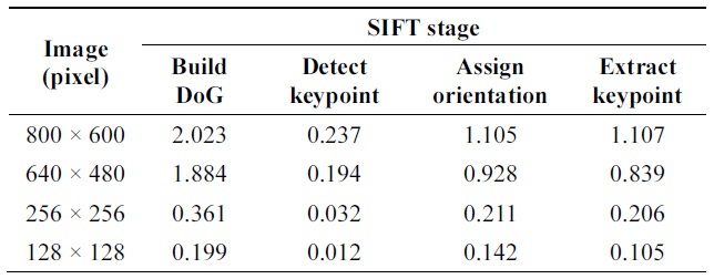
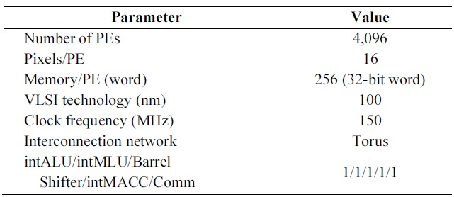
To evaluate the performance of the proposed algorithm, we use a cycle-accurate SIMD simulator. We developed the P-SIFT algorithm in the respective assembly languages for the SIMD processor array. In this study, the image size of 256 × 256 pixels is used. For a fixed 256 × 256 pixel system, because each PE contains 4 × 4 pixels, 4,096 PEs are used. We summarize the parameters of the system configuration in Table 2.
System parameters
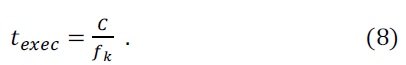
The metrics of execution time and sustained throughput of each case form the basis of the study comparison, defined in (8) and (9):
Execution time
Sustained throughput
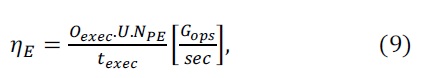
where
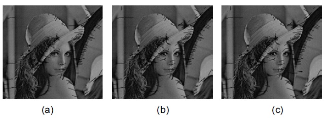
Fig. 9 shows the detected SIFT features in the case of a Lena image. As the number of scales increases, the detected SIFT features become more precise.
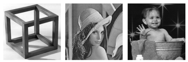
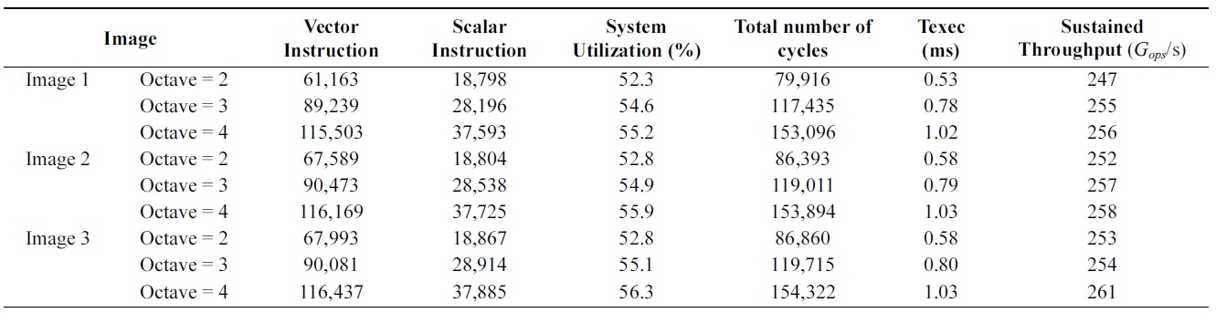
In this experiment, we use three different images (1, 2, and 3) as presented in Fig. 10. The number of octaves is also changed to 2, 3, and 4 in order to evaluate the complexity of the SIFT algorithm.
Table 3 summarizes the execution parameters for each image in the 4,096-PE system. Scalar instructions control the processor array. Vector instructions, performed on the processor array, execute the algorithm in parallel. System Utilization is calculated as the average number of active processing elements. The algorithm operates with a System Utilization of 54% on average, resulting in a high sustained throughput. Overall, our parallel implementation supports sufficient real-time performance (1.03 ms) and provides efficient processing for the SIFT algorithm.
[Table 3.] Algorithm performance on a 4,096-PE system running at 150 MHz

Algorithm performance on a 4,096-PE system running at 150 MHz
[Table 4.] The distribution (measured in %) of vector instructions for the algorithm
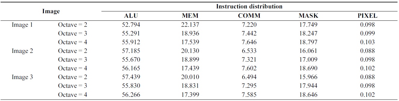
The distribution (measured in %) of vector instructions for the algorithm
Table 4 shows the distribution of vector instructions for the parallel algorithm. Each bar divides the instructions into the arithmetic logic unit (ALU), memory (MEM), communication (COMM), PE activity control unit (MASK), and image loading (PIXEL). The ALU and MEM instructions are computation cycles, while the COMM and MASK instructions are necessary for data distribution and synchronization of the SIMD processor array. The results indicate that the proposed algorithm is dominated by ALU, MEM, and MASK operations.
In comparison with previous approaches, we implemented the experiment for a 640 × 480 pixel image. The number of octaves is 4. The calculated execution time after the implementation is 3.07 ms. Therefore, our proposed implementation can process a sequence of 640 × 480 images at
Recent advances in a wide range of applications of the SIFT algorithm in the field of computer vision require an increase in computational throughput and efficiency. These increased demands have become an important challenge in implementing the SIFT algorithm in real-time applications. In this paper, a parallel implementation of the P-SIFT algorithm using block filtering based on a SIMD pixel processor was presented. By using the SIMD pixel processor system, we fully exploited the available parallelism of the P-SIFT algorithm, primarily in the DoG space construction step. The obtained average processing speed was 326 FPS for images with 640 × 480 pixels. In comparison with the previous implementation [8,11], the proposed method was 30 times faster than the GPU and 7 times faster than the multicore implementation. In this research, we simulated the SIFT algorithm in the SIMD pixel processor. From the obtained performance result, we concluded that an actual implementation on hardware promises a good solution to implement the SIFT algorithm in real-time applications. The monolithic design and SIMD operation node allowed the FPS rate to be sustained at variable image sizes. The bandwidth bottleneck between the detector array and parallel processors did not exist even when the image size was increased. The experiment results also indicated that the proposed parallel approach provided a high-throughput, low-memory implementation and reduced the load imbalance.
where
and
Pe(ρ) ? ρ-d
is identical to (4b), and ? is referred to as the exponential equality.
The optimal DMT curve represents the maximum di-versity gain for a given multiplexing gain
satisfies
Pout(R0,ρ) ? ρ-d*(r),
where
In this subsection, we show that the simple instantaneous DF relay scheme achieves an optimal DMT curve. An upper bound on the DMT based on an instantaneous AF relay is also derived for the sake of comparison. We start from the following lemma:
Lemma 1.
and
The proof of this lemma is presented in