Recently, there has been considerable research in the area of motion planning, which is an essential part of almost all robotic systems. Its area of application goes beyond robotics into the areas of computational biology, computer animation, and economics.
Further, in the past few years, the development of automated driving systems has been a source of many challenges for motion planning. Many approaches to solving the problem have been developed and successfully implemented.
The initial motivation for this work was to develop a motion planning algorithm that could drive an autonomous vehicle in an unknown cluttered environment under differential constraints. The development was a part of preparations for Hyundai-Kia Autonomous Vehicle Competition 2012, held in Korea.
Among the recently developed motion planning methods for autonomous vehicles, several types of planning approaches may be distinguished. The most widely used ones are space discretization-based and sampling-based methods. The former methods work well in cluttered environments but have trouble in generating smooth trajectories and taking kinodynamic constraints into account, and vice versa.
The proposed method is based on the idea of simultaneously running two different types of motion planning algorithms, which interact with each other and benefit from each other’s advantages. This approach was studied in [1,2] and applied to offline motion planning with dynamics in a
cluttered environment. In these works, a graph search algorithm runs in a discretized workspace and guides the extension of a tree in a continuous configuration space. The progress of tree extension is then estimated and is utilized to update the extension heuristics of the higher-level path planner.
In our work, we have applied a similar strategy. However, instead of running a discretization-based algorithm in a projection space, we introduced a simple method that propagates an artificial wavefront, which helped us to resolve some issues with the resolution of a projection space discretization. It allowed us to run the planning algorithm in real time. Simultaneously, we noticed that the generated wavefront may be utilized to construct a potential field with no local minima, which converges in the initial point. This field may later be utilized to produce a navigation function [3]. However, navigation function for this particular problem is not studied in this paper.
Navigation functions open more opportunities for the feedback motion planning, where a separate pathfollowing controller is not required. Of greater significance is the fact that in conjunction with reactive planning algorithms, these functions allow the creation of planners that can cope with unpredicted dynamic obstacles in unknown environments.
Works on Euclidean shortest paths include [4,5]. Unlike methods based on interpolation, the proposed wavefront propagation method is based on random sampling, performs a feasibility check not only on the obstacle presence but also on the kinodynamic constraints of the robot, and easily integrates with a sampling-based motion planner.
One of the common approaches in the area of motion planning is to discretize the configuration space and then run a graph-search algorithm like A* or Dijkstra’s algorithm. This approach was applied to solve the problem of autonomous vehicle driving in [6,7].
Some other works (rapidly exploring random tree [RRT] and probabilistic roadmap [PRM]) [8,9] introduce approaches for motion planning in continuous space with kinodynamic constraints. Unlike methods with space discretization, these methods suffer less from the so-called curse of dimensionality, when the algorithm complexity increases exponentially with the number of dimensions. Further, these methods can generate smooth trajectories, which do not require additional smoothing or optimization [6]. However, depending on the environment (presence of narrow paths), these methods may run for an indefinitely long time. To overcome these issues, many strategies for sampling biasing have been introduced [10,11].
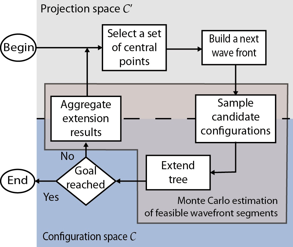
The proposed method combines a sampling-based motion planning method and an artificial wavefront propagation method (Fig. 1). The sampling-based algorithm is run in a full configuration space
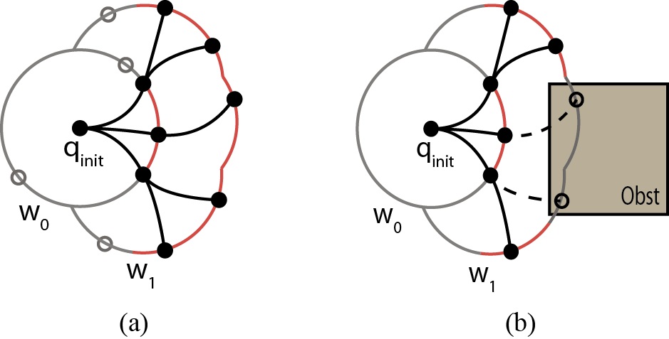
A sampling-based planner is a type of rapidly exploring dense tree (RDT) algorithm. It manages the kinodynamic constraints check and the obstacle collision checks by means of a simulation. The sampling is biased by an artificial wavefront, which propagates in a projection space. After the tree is extended to the configurations sampled at the current wavefront, the progress of the propagation is analyzed, and the center points for the construction of the next wavefront are determined.
We consider the wavefront as a curve or a set of curves in a two-dimensional space or a surface or set of surfaces in a higher-dimensional space.
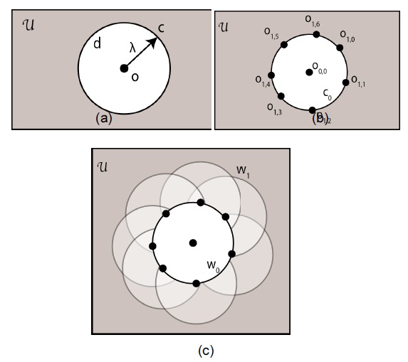
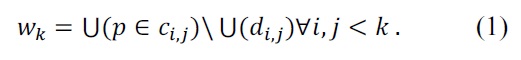
To describe the wavefront construction, let us introduce two variables
We then utilize an idea from Huygens principle that every point where the wave has reached becomes a source of secondary waves. However, following the original Huygens principle would imply an infinite number of points. There-
fore, in our case, we limit the number of points. Let us now sample several points
Then, we construct overlapping circles
At the next step, new center points
Such a definition of a wavefront gives us several advantages:
Even if just one center point is sampled for the construction of the next wavefront, the wavefront may still be constructed.
Normals to the wavefront point to the corresponding center points and thus to the previous wavefront, converging to the point of the origin.
Points on the wavefront may be sampled with a simple algorithm, described below, even for high-dimensional spaces.
>
B. Wavefront Sampling Algorithm
One of the issues that arise when working with curves or surfaces is how to represent them. A helpful feature of the proposed wavefront propagation method is that a wavefront is defined only by a set of center points
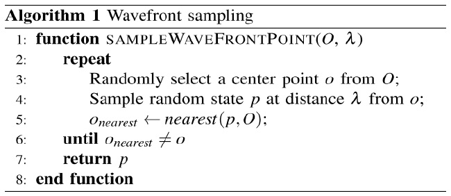
The sampling function is shown in Algorithm 1. First, it samples random points on all circles and then, filters those, which do not overlap any of the open disks. The function
For the completeness of the sampling-based motion planner, it is important for the sampled sequence to be dense. Let us consider an approach that makes the proposed artificial wavefront a dense sequence.
There are two parameters that affect wavefront con-struction:
Theorem 1.
Theorem 2.
As the wavefront is the boundary of
Theorem 3.
In the proposed method, a sampling-based planner runs synchronously in a full configuration space
generates a plan for execution;
ensures the feasibility of paths by means of constraints and obstacle collisions checks; and
provides the means to simulate the propagation of the system to the next wavefront.
The sampling motion planner is based on a RDT (also known as RRT) [2]. An important feature of the RRT planner is its probabilistic completeness in the case of a dense sampling sequence. It uses a tree to represent a set of generated paths, where nodes correspond to configurations, and edges correspond to the feasible paths between configurations. The tree is iteratively extended towards sampled configurations unless the target or a certain limiting condition is met. In the proposed method, candidate configurations are sampled on the wavefronts, as shown in Fig. 3.
Let the tree be denoted as
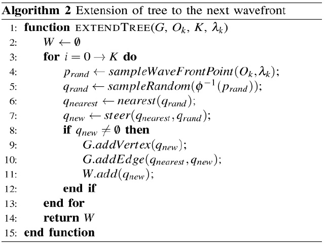
The tree extension procedure is shown in Algorithm 2. It is similar to that of RRTs, except the random sampling part. First, a point
After a candidate is sampled, the nearest configuration in the tree is selected. Then, the algorithm attempts to connect the closest configuration to the candidate configuration with a valid collision-free trajectory by means of simulation. If kinodynamic constraints are maintained (Fig. 3(a)) and the paths are obstacle free (Fig. 3(b)), then the candidate state and the linking path are added to the tree.
Propagation is performed in stages, wavefront by wavefront, and at every stage, some limited number of iterations is performed. For the proposed system, we determined this parameter experimentally by choosing between the smoothness of the path and the available computational resources.
After each stage, configurations that were successfully added may be considered as the representatives of the feasible segments of the current wavefront. This set of configurations is then analyzed to determine the shape of the next wavefront.
>
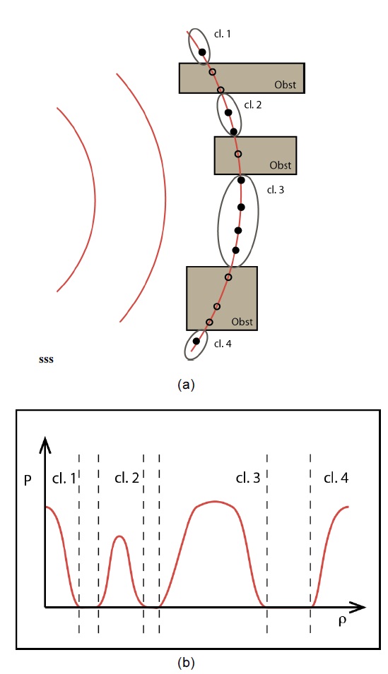
E. Stochastic Analysis of Expansion Progress
When new candidate points are sampled at a new wavefront, which parts of the new wave front are feasible and which ones are not is not known. The complete solution to determine, which wavefront segments are feasible, may
not exist because obstacles in the considered space may have various shapes. From the other side, the tree null, of the sampling-based planner, extends only to feasible configureations. Therefore, a tree extension may be considered a tool for the stochastic estimation of the feasible segments of a wavefront.
From there, we can pick the center points
Let us propose some variable
When we apply a tree extension, we may notice that
In order to determine
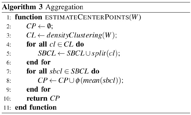
Algorithm 3 shows how propagated configurations are aggregated. The function
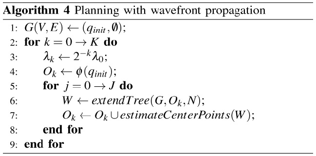
Algorithm 4 shows the main routine of the proposed method. The algorithm works by consecutively propagating a wavefront. It gradually increases the resolution to achieve the sampling density and thus the planner completeness. It should be noted that the tree
the resolution limit,
The initial motivation for the development of a motion planner was participation in a national autonomous vehicles competition held in Korea. We implemented a multithreaded version of our algorithm and integrated it into an autonomous vehicle. We then performed several tests in a simulated environment in order to compare our method to other related motion planning algorithms, and to investigate the wavefront behavior in a variety of environments. We also tested our motion planner on an autonomous vehicle, driving it through obstacle patterns difficult for a samplingbased planner.
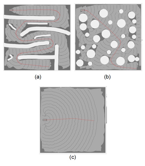
To estimate the performance of the developed method, we ran a simulation in different types of environments: in a narrow labyrinth, with scattered obstacles, and with no obstacles (Fig. 5). We ran each algorithm ten times on a laptop with quad-core CPU and measured the computational time. Algorithms were made to run in parallel, with shared memory.
We compared our approach to a modified RRT algorithm, because it was already tested on a real autonomous vehicle, and to an algorithm based on Kinodynamic Planning by Interior-Exterior Cell Exploration (KPIECE) algorithm, because our approach is similar to the idea of combining two different planning algorithms.
To generate a sufficiently smooth path, we applied an approach, which was utilized in RRT* [12] and included cost-to-go into the distance for the nearest-neighbor search. Optimization was performed on time and lateral and longitudinal accelerations. Hence, we did not compare our results to the original KPIECE [2] or SyClOP [1] planners, as these planners utilize a forward dynamics simulation, lack the nearest-neighbor search, and have limited capability of increasing the optimality. Nearoptimal paths are important for driving at relatively high speeds. Although we do not claim optimality convergence in the proposed method, the main goal was to create trajectories that were sufficiently smooth for high-speed driving.
We implemented a nearest-neighbor search-based algorithm and applied a sampling strategy similar to KPIECE.
We ran a discretization-based planner in the projection space and biased the sampling to the boundary region between the explored and the unexplored zones. For the experiments, we labeled this method as nn-KPIECE.
The results are presented in Table 1: average, minimum, and maximum algorithm run times were recorded. From these results, it can be concluded that ODEx performs considerably better on narrow paths, approximately similar to RRT in an environment with scattered obstacles, and RRT performs better in an open environment. The other advantage of ODEx is that the computational time is considerably less random in comparison to RRT. In comparison to nn-KPIECE, our algorithm performed slightly
[Table 1.] Comparison of run time in different environments
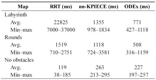
Comparison of run time in different environments
faster but in the same order. The performances of KPIECE and SyCLOP are influenced by the cell size in discretization- based high-level planners. This is one of the disadvantages of these methods, and probably, the cell size was not optimal during the experiments.
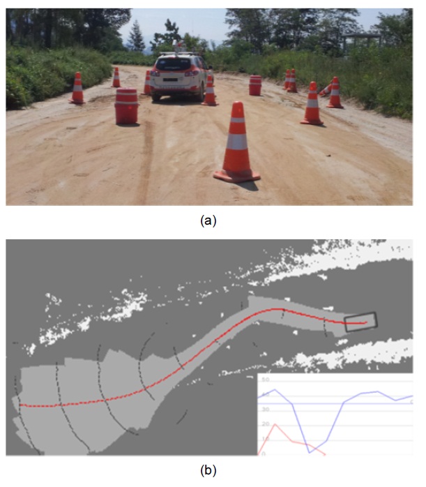
We performed various tests in a real environment. One of the most challenging tests for an autonomous vehicle is navigation in narrow passages, which are difficult for sampling-based motion planners. In the test, we placed road cones in a grid pattern; the distance between the cones was approximately 4?6 m in Fig. 6(a). Our planner generated a trajectory in real time from the map updates, which were generated with the readings from laser scanners in Fig. 6(b). The graphs of curvature and speed profiles are also shown. The speed was not high, as we applied the speed-dependent width of a car for the collision checker in order to compensate for the inaccuracy of the motion controller at high speeds. The initial propagation step
On relatively wide paths, we tested the vehicle by driving at speeds of more than 60 km/h. Planning was carried out considering constraints on lateral and longitudinal accelerations, minimum turn radius, and maximum allowed speed. Dynamics with a side slip was not considered. Depending on the difficulty of the obstacles, the planning time varied from 90 to 600 ms.
During preparations for a national autonomous vehicles competition, we developed a new motion planning approach and implemented it in a real system. We tested the system in a real environment at speeds more than 60 km/h.
The proposed planner solves a combination of planning challenges, including online planning, multiple dimensions, presence of narrow paths, kinodynamic constraints, and unknown environment.
The efficiency of the proposed algorithm was shown experimentally by comparing the performance of the proposed algorithm to that of other planning algorithms in a simulated environment.