III. TWO-STEP JOB SCHEDULING SCHEME BASED ON PRIORITY
The proposed scheduling scheme in this paper is composed of two steps. In the first step, the priority of a job is calculated based on the degree of importance of each job. In the second step, the algorithm selects a VM on which to run the job. Every candidate VM is weighted using the AHP model.
>
A. First Step: Job Classification Based on Its Degree of Importance
As all resources in cloud computing are dedicated to jobs, it is advantageous for a cloud system to secure the resources needed in advance. In the case of data-oriented jobs, this resource provisioning will be an especially important factor in performance improvement because the required storage as well as bandwidth increases with time passing. Thus, our scheme classifies all jobs into one of two categories: resource provisioning or best effort.
In this step, the jobs for which the user pays a high cost or that are of higher importance belong to the resource provisioning case. If scheduling failures of jobs may bring about severe business loss, the jobs are classified to the first level of priority or the highest level. If the failures may cause considerable after-effects, these jobs belong to the second level of priority. Jobs for which the user pays regular or low costs or are of medium importance belong to the best effort case. If scheduling failures of jobs may bring about a trivial inconvenience to a small number of users, the jobs are classified into the third level of priority. If the failures may cause minor functional impairments, these jobs belong to the fourth level or the lowest priority. The classified jobs are queued in order in the cloud system scheduler. The sequences are fixed, and the jobs are executed in a nonpreemptive way. The jobs with the same priority are served in a round-robin manner.
>
B. Second Step: Job Allocation to VM Based on the AHP Model
The AHP is a kind of MCDM that helps to choose one of the alternatives. Each selection has a related attribute attached to it, and the weights of each attribute are set. Therefore, the AHP model can select the best choice out of the list of alternatives. The merit of the AHP is that it considers variable parameters for many alternatives and generates the result that best matches the parameters [10]. The proposed scheme uses an AHP model for the VM selection.
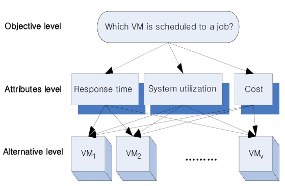
As Fig. 1 shows, the objective level in the proposed algorithm is to place a job in a VM that it best matches under many different parameters. The attribute level in our algorithm is composed of user requirements or decision criteria such as response time, system utilization, and cost, and the alternative level represents all VMs in a cloud system.
As each parameter in the AHP model has a preference, the proposed scheme also has a preference from 1 to 9. The preference 9 is the highest one. The values 2, 4, 6, and 8 are intermediate values for the preference, and the inverse number represents the counterpart preference. Therefore, these preference values are used in representing and calculating the requirements of the job as well as parameters of each VM, such as the response time, system utilization, and cost.
Suppose that a set of jobs, which are scheduling objects in cloud environment, is
The VM allocation is done in two steps. In the first step, the algorithm calculates the weight vector by pairwise comparison and does a consistency check for both of the levels. In the second step, the best VM is selected by multiplying the two weight vectors of each level. The process is explained in detail below.
Sub-step 1: Calculation of the weight matrix and consistency index between the objective and attribute level.
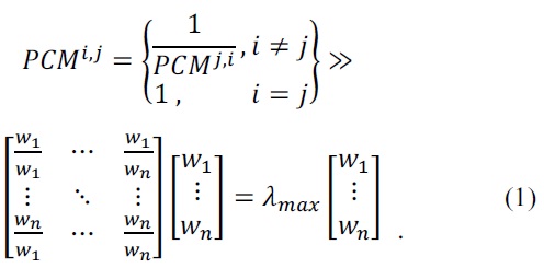
Suppose that the pairwise comparison matrix between the objective level and attribute level is named “pairwise comparison matrix (PCM)” in this paper. This PCM represents the preference for a job under all criteria such as responsiveness, system utilization, and cost. The PCM is an n by n matrix like Eq. (1). If the element of PCM, (

Saaty [10] has defined the consistency ratio (CR) as Eq. (3).
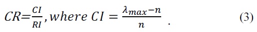
In Eq. (3), RI is the random index, which is randomly calculated based on the rank of the comparison matrix. Eq. (3) also uses the RI values, which were calculated by Saaty [10]. If CR < 0.1, then the PCM should be considered consistent.
Sub-step 2: Calculation of the weight matrix and consistency index between the attribute and alternative level.
The next step is also to calculate the weight matrix and consistency index for each decision criterion to all VMs. Like Eqs. (1)?(3), this scheme determines the pairwise comparison matrix and calculates the weight matrix and consistency ratios for each of the decision criteria to each VM.
Suppose that the weight vector for each VM is

where {ω
IV. ANALYSIS AND EXAMPLE OF THE PROPOSED SCHEDULING ALGORITHM
First, we analyze the proposed scheme by time complexity. As the priority classification of the first step is determined by job characteristics or requirements, the time complexity may be trivial. The computation of the pairwise comparison matrix and CR occupies a huge portion of complexity in the proposed scheme, such as Eq. (5).

In Eq. (6),

The time complexity for multiplying
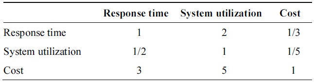
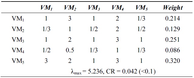
The following is an example of the proposed scheduling algorithm. Table 1 is a sample preference matrix of a job.
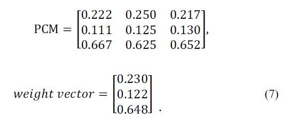
The following Eq. (7) is a PCM and weight vector.
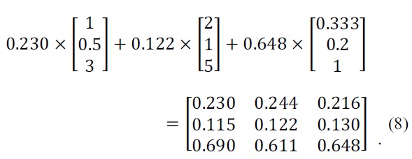
For obtaining the CR, we first multiply the preference matrix by the eigenvalue of the weight vector as shown below Eq. (8):
From Eqs. (2) and (3), we now can get the
[Table 1.] Preference matrix example of a job

Preference matrix example of a job
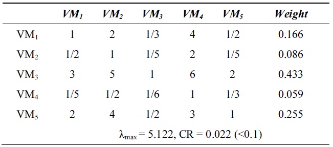
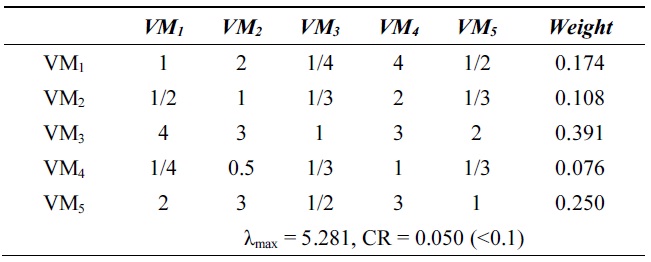
[Table 2.] λmax and consistency ratio (CR) for response time

λmax and consistency ratio (CR) for response time
[Table 3.] λmax and consistency ratio (CR) for system utilization
λmax and consistency ratio (CR) for system utilization
[Table 4.] λmax and consistency ratio (CR) for cost
λmax and consistency ratio (CR) for cost
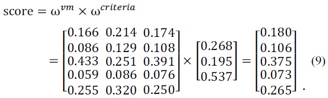
Finally, the score of each VM is calculated by multiplying the weight matrix (ω
Next, we calculate the weight vector and CR of each VM for the response time, system utilization, and cost. Tables 2?4 show these weight vectors and CRs. As all CRs are less than 0.1, all preference matrices must be consistent.
Job scheduling is an important problem in cloud computing, which is naturally composed of heterogeneous resources. We defined this issue as MCDM. To settle this issue, this paper introduced a two-step job scheduling scheme based on priority, with consideration of both the job characteristics and the MCDM. In the first step, the priority of a job was classified in 1 of 4 levels, which are determined by importance attributes. In the second step, we applied the AHP process in job allocations to the VM to tackle the MCDM issue. We adopted responsibility, system utilization, and cost of jobs as decision criteria. We then analyzed the time complexity of the proposed scheme and confirmed that the proposed algorithm showed acceptable complexity. In the future, work will be carried out aiming to minimize the complexity and to implement a real scheduler in a sample cloud system.