The analysis of multi-dimensional two-phase flows has become a very challenging topic in many thermal hydraulic applications such as nuclear reactor safety. In particular, during a postulated large break loss of coolant accident (LBLOCA) period, the multi-dimensional behavior of a two-phase flow is expected to occur at several regions in the system, which significantly affects the key safety parameters. (Chung B.D. et al., 2007)

For the past several decades, safety analyses for nuclear systems during a transient period have been performed based on a one-dimensional approach. Even when strong multidimensional flow characteristics were expected during the transient, the safety was analyzed one-dimensionally by adopting sufficiently conservative assumptions for the important phenomena or by controlling the physical parameters. However, a safety analysis code based on a onedimensional concept has a fatal limitation in its application to a multi-dimensional two-phase flow since it can adapt inappropriate physics in terms of flow structure, dynamic interaction between phases and so on.

Recently, along with the enhanced capacity of the computational fluid dynamic (CFD) code and advances in computing technology, interest in multi-dimensional flow phenomena has increased. Based on a recent trend of safety analyses for nuclear reactors, a new system analysis code, called SPACE, has been developed based on a two-fluid, three-field model (Kim et al, 2009). SPACE has the capability of a multi-dimensional flow application at the component scale. To validate the performance of SPACE, a lot of experimental data are required for the validation of various thermal hydraulic models as well as the verification of them.

However, a very limited number of experiments have been found in the literature for a large scale of well-defined multi-dimensional flow. Bukhari and Lahey Jr. performed a two-dimensional experiment with a test section having slab geometry of 0.91×m×0.91 m×0.0127 m (Bukhari et al., 1987). Void fraction data were taken at 27 locations of the slab plate. A single-beam gamma ray attenuation technique was used to determine the void fraction distribution within a 2-D test section for various boundary conditions including a recirculation flow condition. Although the literature shows a good applicability of the code validation for a multi-dimensional capability, the present work focuses on phenomena that possibly occur in a downcomer having a relatively larger gap. Acquiring a void fraction profile with a better resolution is another motive of the current study. The present study focused on a conceptual problem of the slab geometry having a sufficiently large gap, reducing the wall shear effect of individual cap/slug bubbles.

Several measurement techniques have been used for characterizing the void fraction of a two-phase system: the conductance probe method, the radiation attenuation method using a gamma densitometer or X-ray, and the impedance method. Among them, the impedance method is very practical in terms of the non-intrusiveness of the sensors, a relatively simple measuring principle, and reasonable costs for the signal processing (Delhaye et al., 1987). Its measuring principle is generally based on the differences of impedance of a two-phase mixture owing to a variation of void fraction around the void sensor. The impedance method can be classified into two categories, depending on the liquid material selected: an electrical conductivity method and a capacitance method. The electrical conductivity method uses a conducting material like water to measure the void fraction of the two-phase flow. It can also be used to measure the water level and liquid film thickness. The capacitance method is used to measure the void fraction in two-phase systems in which the liquid is a non-conducting material such as a refrigerant or oil. (D. Barnea et al.1980, H.C.Kang et al., 1992, C.-H. Song et al., 1998, H.C.Yang et al., 2003)

The purpose of the current study is to generate an experimental database for multi-dimensional two-phase void distribution to validate the performance of the safety analysis code, SPACE. Since SPACE was designed as a system scale code, the data should represent the system scale behavior. Another purpose is to develop a high performance impedance measuring system for the system scale geometry of a two-phase system.

The present study focuses on the quantification of an adiabatic two-dimensional flow in large slab geometry with definite boundary conditions. For this purpose, a test facility, called DYNAS (a test facility for DYNamics of Air/water System), was newly designed and constructed. Two separated test sections were prepared for the visualization and impedance measurements, repectively. The shape and scale of the test section points to the phenomena of twophase multi-dimensional behavior at the downcomer region, which are thought to occur during a loss of coolant accident. The phenomena of interest were simplified and characterized under low pressure air/water conditions since the focus of the current study is not on the nuclear system performance but on the quantification of the multi-dimensional behavior to evaluate the performance of the currently developing safety analysis code.

The DYNAS facility has a test section with slab geometry of 1.43 m×1.43 m×0.11 m, which was made of 60 mm thick acrylic plates. Various kinds of two-dimensional flow patterns were simulated using different opening combinations of the inlet and outlet nozzles. The major parameters measured were the two-dimensional void fraction profile in the slab type test section as well as the thermal hydraulic boundary conditions. The void fraction was converted from the impedance measured between two electrodes installed on the inner surfaces of the slab acrylic plates. Experiments were performed at lower pressure and at 35 ℃. Various flow rates of water and air were set to obtain data representing dynamic multi-dimensional two-phase movement. For each selected inlet and outlet nozzle combination, the water flow ranged from 2 to 20 kg/s, and the air flow rate ranged from 2.0 to 20 g/s, which correspond to 0.4 to 4 m/s and 0.2 to 2.3 m/s of superficial liquid and gas velocities based on the inlet port area, respectively.

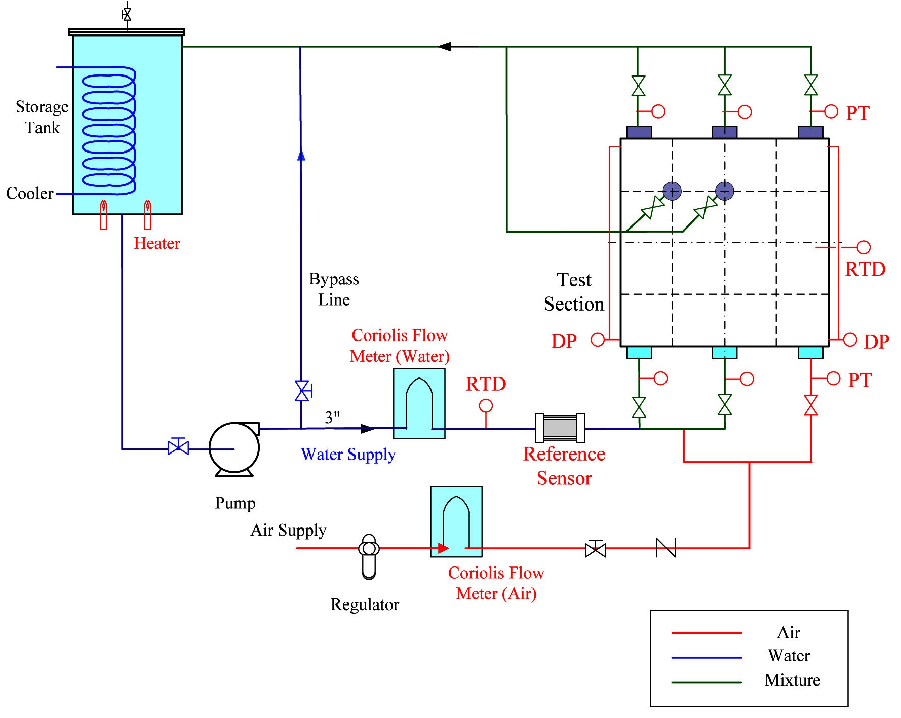
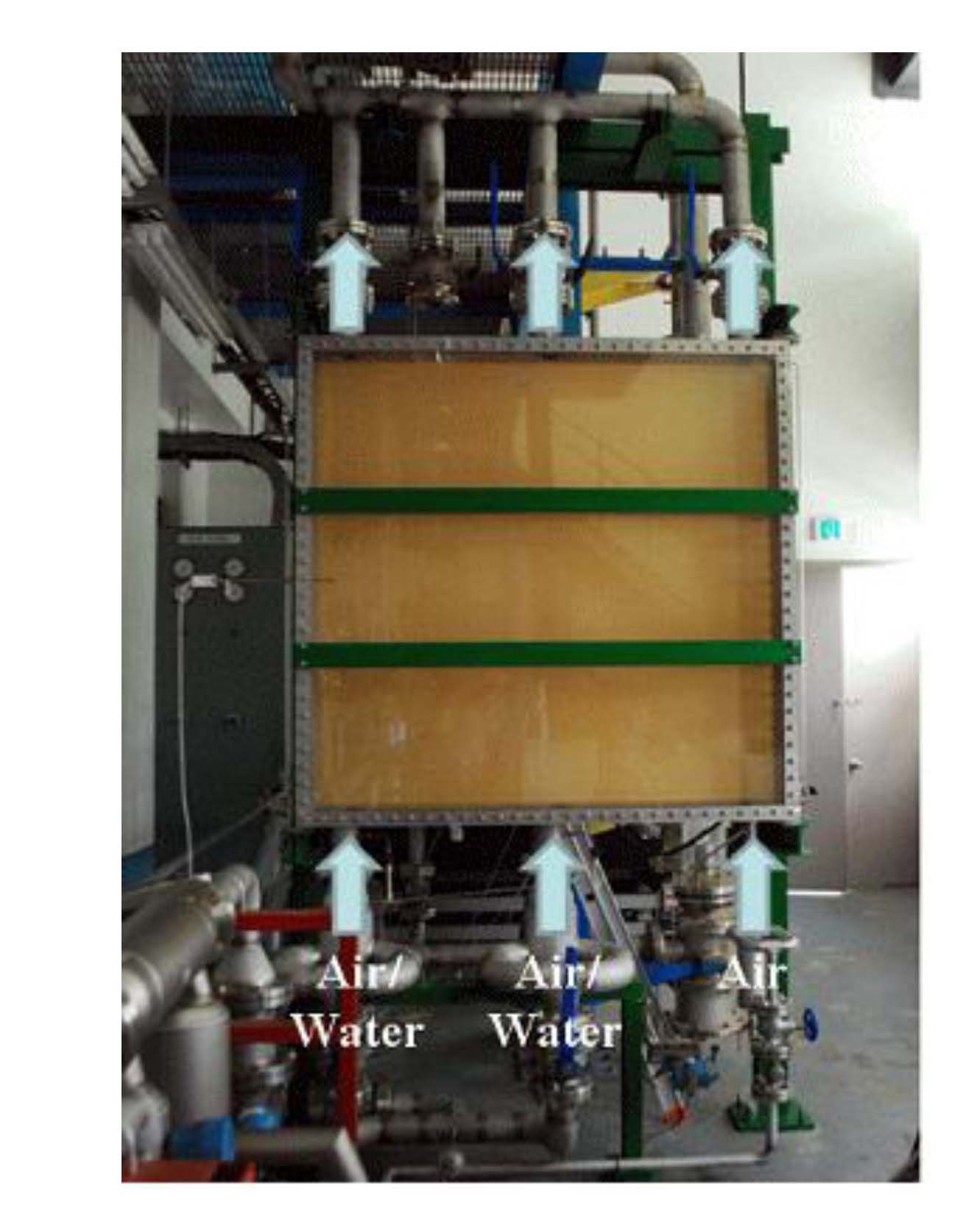
Figure 1 shows a schematic of the experimental apparatus, called DYNAS. The fluid system consists of a test section, a storage tank, and a piping system for the water and air supply to the test section and return back to the storage tank. The storage tank was installed at the top part of the facility, where the air in the returned two-phase mixture flow was separated. The water temperature in the system was controlled using a cooler and heater imbedded in the storage tank. The water flow was supplied using a centrifugal pump with a 92 m head and 100 m³/hr capacity, which was controlled by adjusting the impeller speed using an inverter. A bypass line was established at the upstream of the test section for an efficient control of the water flow. In the water injection line, instrumentations for the flow rate, temperature, and pressure were installed. A reference impedance sensor was installed at the inlet of the test section in the water supply system, of which the impedance value was utilized for compensation of the void fraction

at each point of the test section. Air was supplied to the test section from a compressor, which was maintained at 6 gauge bars. A regulator controls the air injection pressure before the air is delivered to the test section.

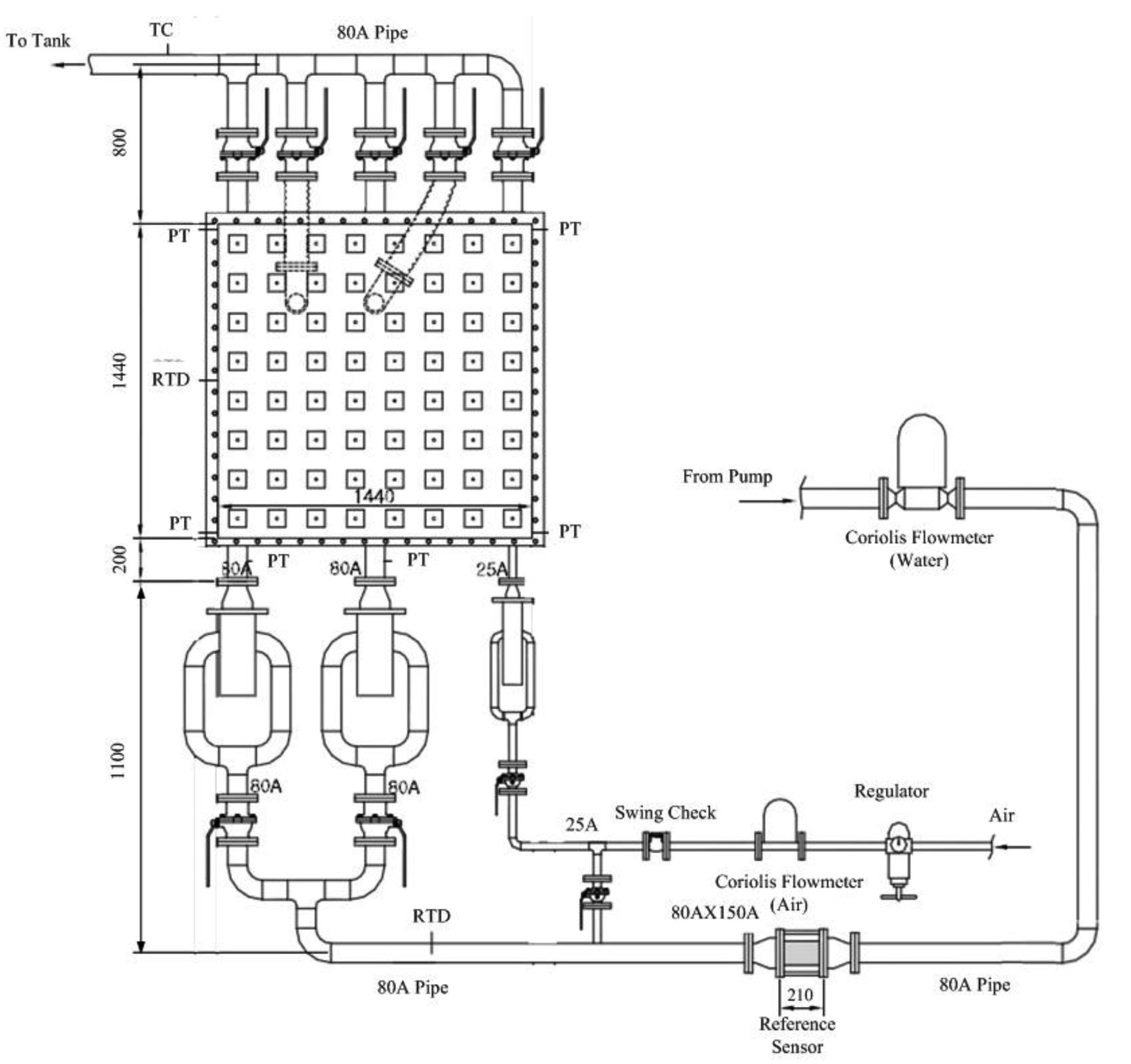
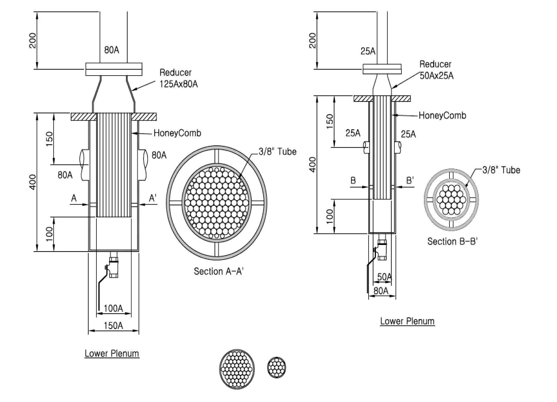
Figure 2 shows the design features of the test section and the important components. The two-phase flow injected through the selected inlet valve was split into two streams and gathered at a common header. The flow goes downward in the annulus inside the common header and enters the test section through the inlet nozzle. To maintain a straight flow at the inlet, a flow straightener and honey vane were installed inside the inlet pipe. Figure 3 shows the internal design of the test section inlet pipe. The inlet structure also contributes to the flow stabilization by supplying hydraulic resistance in advance of the injection into the test section, especially for a low flow condition.

The present study focuses on the hydraulic behavior of a nuclear reactor downcomer having a 0.25 m gap size. Such a relatively large channel prevents the formulation of a slug bubble plugging the whole channel. Since the small gap geometry of the test section can bear undesirable wall shear momentum loss induced by a slug bubble, the test section was designed to have a gap scale greater than the stable maximum bubble size, which can be analyzed using the following formula (Kataoka et al., 1987):

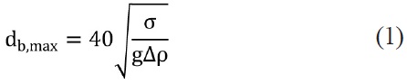
From the above analogy, the gap scale between the two slabs was determined to be 0.11m by referring to the air and water properties at room temperature. Two test sections were manufactured for a measurement of the impedance at the local points of the test section, and a visualization of the overall flow characteristics of a twodimensional flow. Two independent tests for the same flow conditions were performed with different test sections

corresponding to measurement methods. The visualization test serves as a qualitative benchmark of the void profile results from the impedance measurement method. Both of the test sections have a dimension of 1.43 m×1.43 m ×0.11 m based on the internal fluid volume. Each plate composing the slab geometry was made of a transparent acrylic plate. Support bars were installed on both faces of the acrylic plates to prevent inflation induced by the hydrostatic water head. A steel frame was designed to support the weight of the fluid and the acrylic structure.

To perform a visualization test, transparent acrylic plates and minimum support bars were used to obtain the flow pattern and qualitative void and velocity distributions. Although the thickness of the acrylic plate is 30 mm, Itype beams were installed to prevent inflation occurring owing to the large size of the slab and the hydraulic force of the internal water. Figure 4 shows a section of the facility near the test section for visualization.

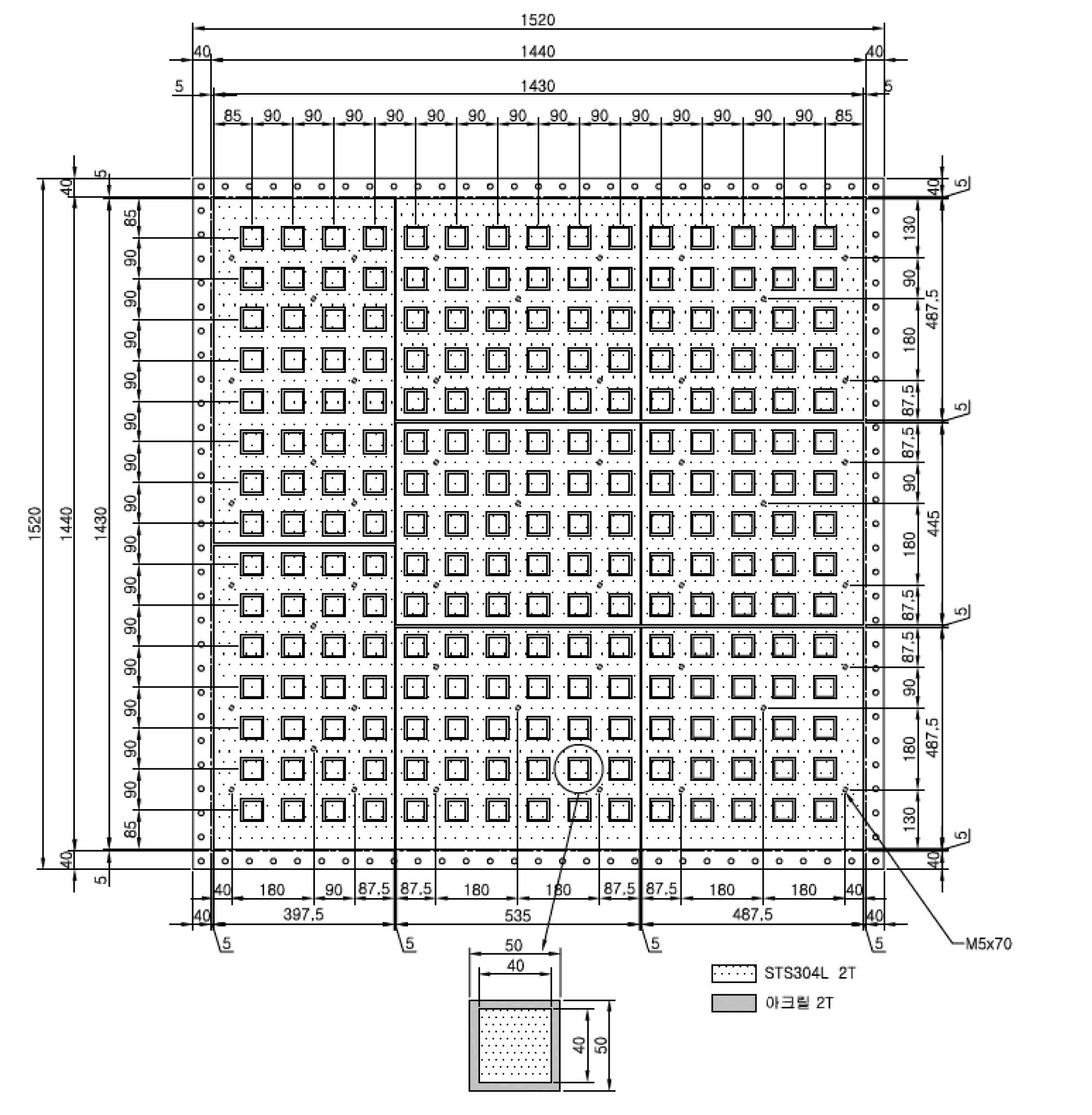
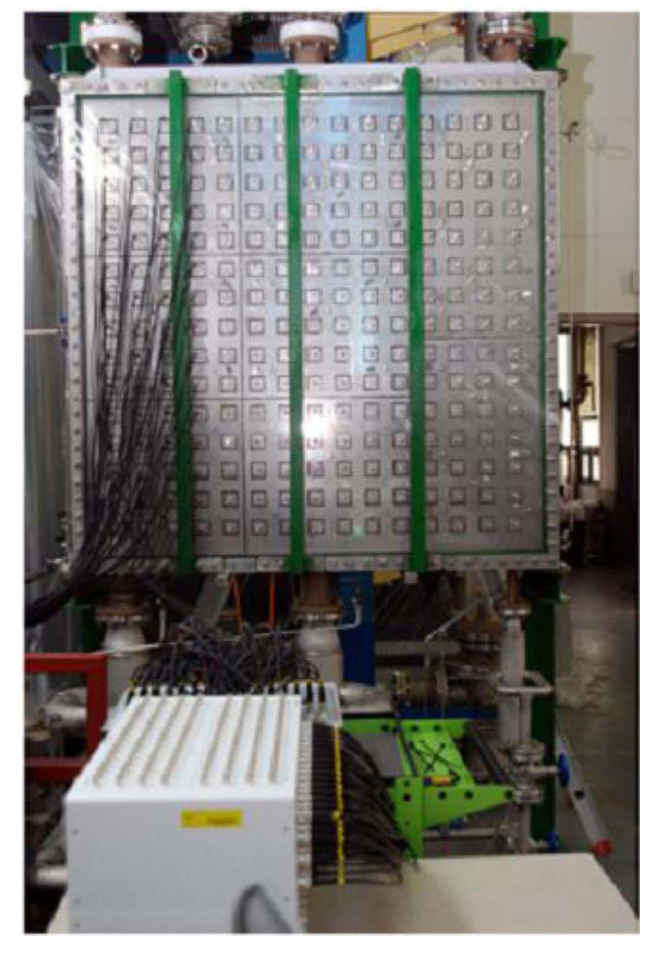
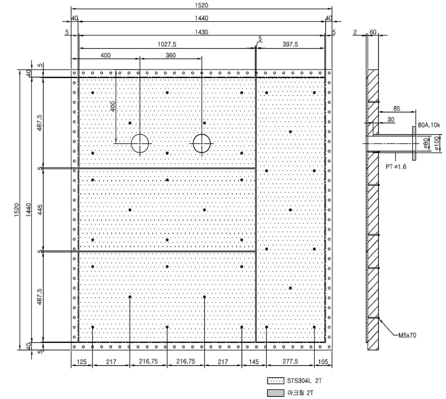
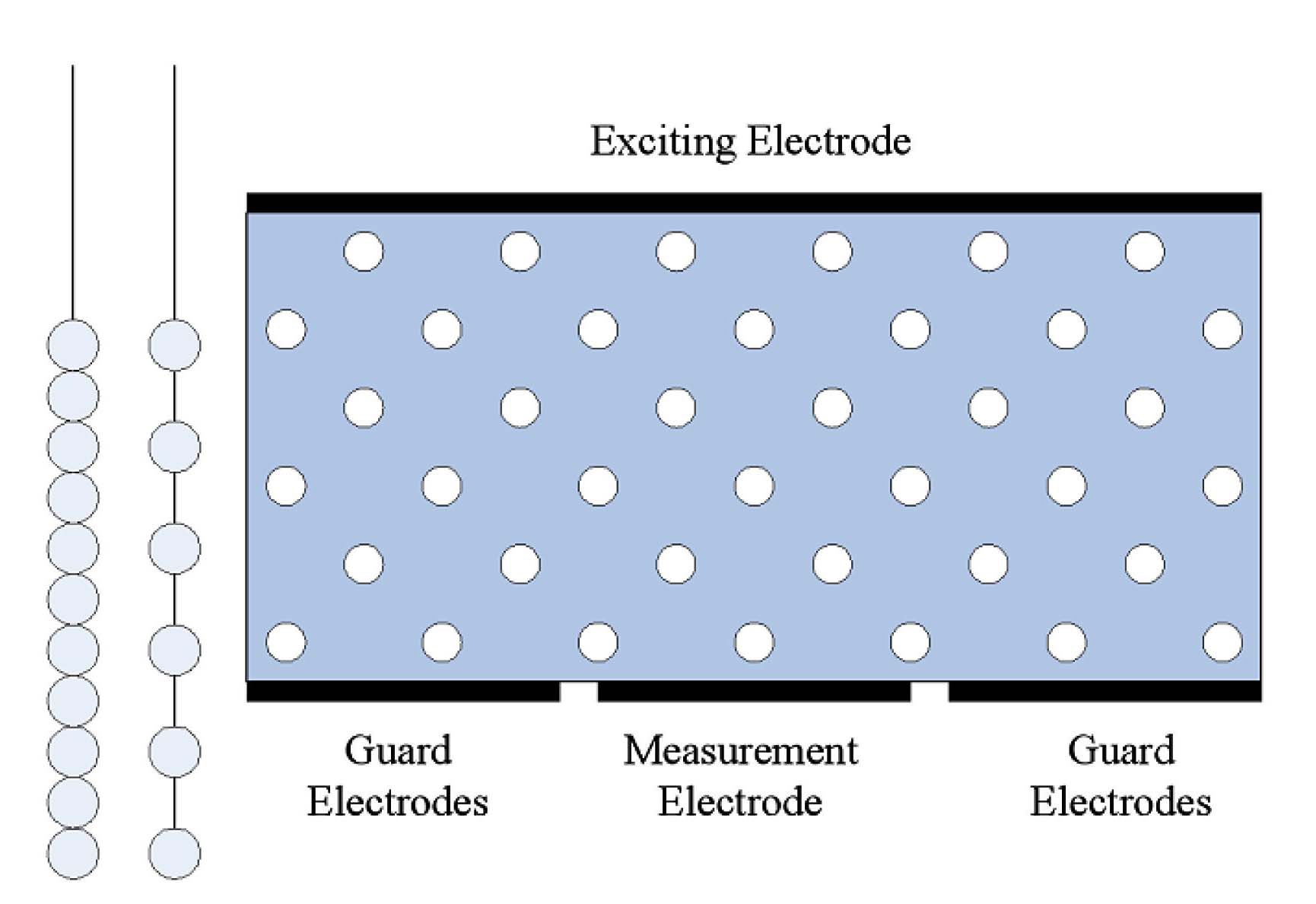
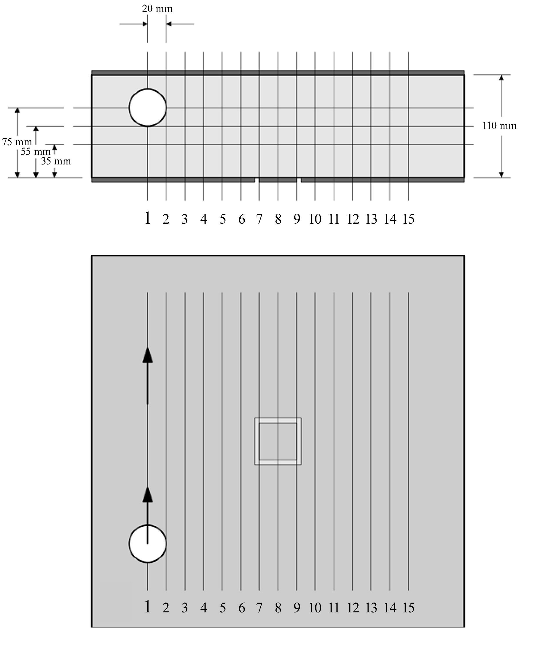
The test section for the impedance measurement has 15×15 electrodes, each of which has a dimension of 4 cm×4 cm. The local void fractions in the test section were obtained by measuring the impedance between two electrodes installed face to face on each inner surface of an independently manufactured test section, as shown in figure 5. The space between the sensing electrodes was filled with a stainless steel plate that serves as a guard electrode to form a straight electric field. The sensing

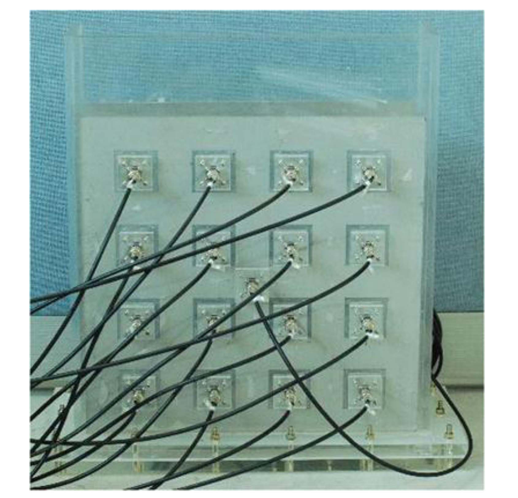
electrode and guard plate are separated by 5 mm for insulation, the space of which was filled with acrylic pieces to maintain a smooth inner surface. Figure 6 shows a photograph of the test section upon which the electrodes were installed. Some cabling from the measuring systems to the signal conditioner is also shown in the photograph. On the inner surface of the opposite side plate, four large thin plates were installed as shown in figure 7, which are electrodes supplying an electric potential.

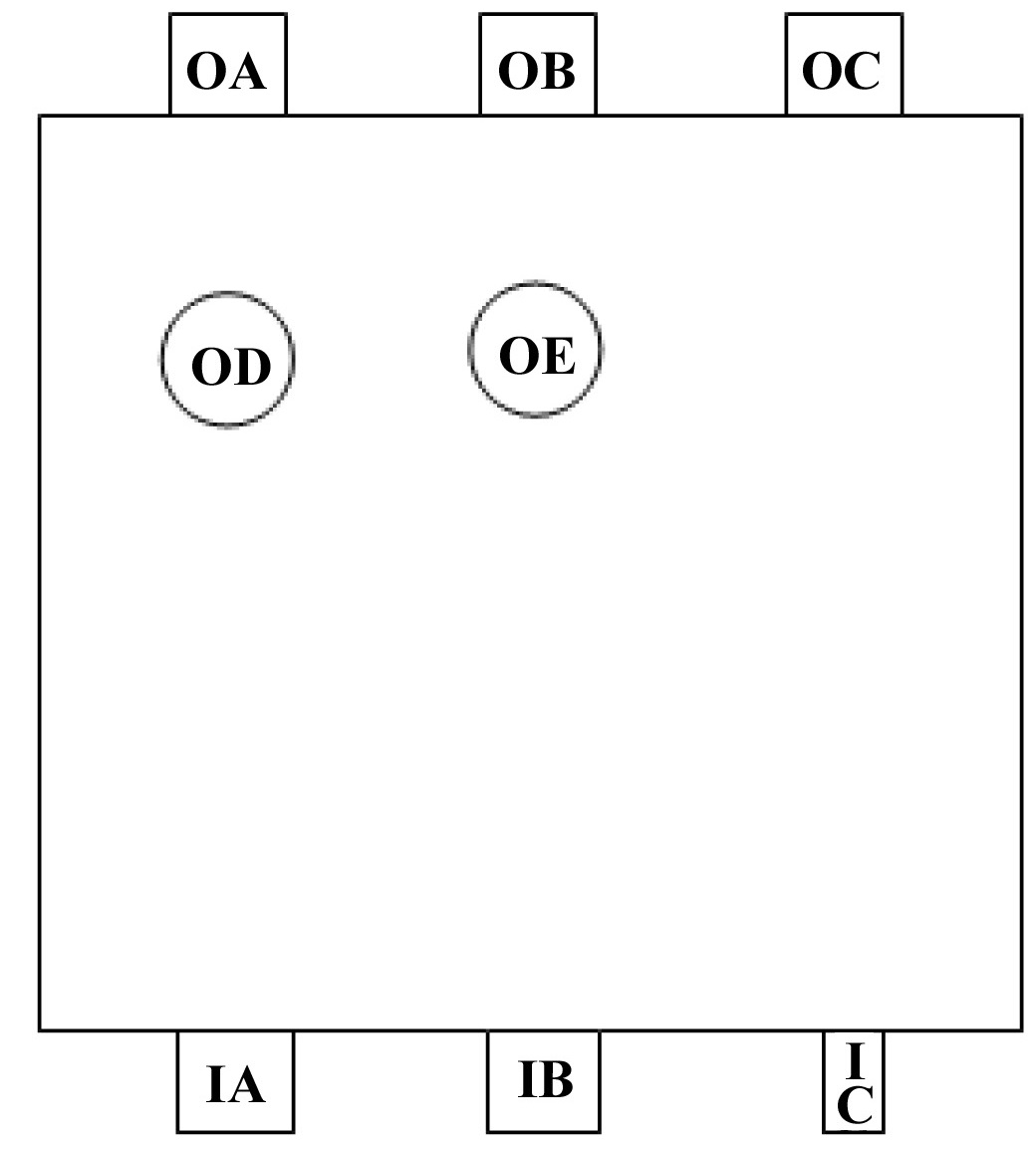
The test section has three inlet and five outlet nozzles. The size of each nozzle is 3” except for the air inlet nozzle, which was connected only to the air supply line (See figure 2). Through the other two inlet nozzles, a singlephase water flow or two-phase mixture flow can be supplied.

Three outlet nozzles were installed on the top face of the steel structure, while two outlet nozzles were installed on the face of an acrylic plate. Using the latter two nozzles, a conceptual flow pattern in a downcomer near a postulated broken cold leg during a loss of coolant accident can be simulated. By selecting a combination of inlet and outlet nozzles, various types of multi-dimensional flow behaviours can be simulated.

In the present study, the combinations of one inlet and one outlet nozzle formed a test matrix. After the test case was selected, engineering plastics were used to fill up unutilized outlet nozzles to make a smooth wall on the inner surface of the test section, and to remove air pockets induced by a stagnant volume between the test section and the outlet valve.

Instrumentation of the DYNAS system can be classified into two categories: (1) instrumentation for boundary parameters such as pressure, temperature, and flow rates of both phases, and (2) local measurement of impedance used to obtain a two-dimensional void fraction.

Several types of commercially available instruments were installed to measure the boundary conditions. The mass flow rate of the injected water is measured using a 3” Micromotion mass flow meter installed at the water supply line. The estimated uncertainty for the measured mass flow was 0.05% of its read value. For a given span, at 27 kg/s, the maximum bias uncertainty has been analyzed as 0.015 kg/s including the DAS uncertainty. An 1” Micromotion mass flow meter was used to measure the air flow at the air supply line with a bias of 0.5% of the reading value. The system pressure was measured at the top and bottom of the test section using two SMART-type PTs (pressure transmitter). The estimated uncertainty of each PT reading was 0.08% of the full scale, including the DAS uncertainty. To measure the temperature of the fluid, two RTDs were installed one at the water supply line and the other at the side of the test section. A Watrow class-A 3-wire standard 0.25” RTD plug type was used. The uncertainty of the RTD was expected to be 0.28 ℃ at 35 ℃. The system temperature was maintained at 35 ℃ by considering the heat generation from the pump at the maximum flow condition and the cooling capability of the loop. By referring to the temperature at the water supply line, the applied power of the heater inside the storage tank was controlled by an SCR.

A visualization of the two-phase dynamics using a transparent test section was performed using a Sony HDCAM (1920×1080 pixels) in continuous mode by using day-light. The frame rate of the recording device was 30 Hz. The field of view was 1500×1800 mm, and the test area was cropped to 400×480 pixels. (Kim et al., 2010)

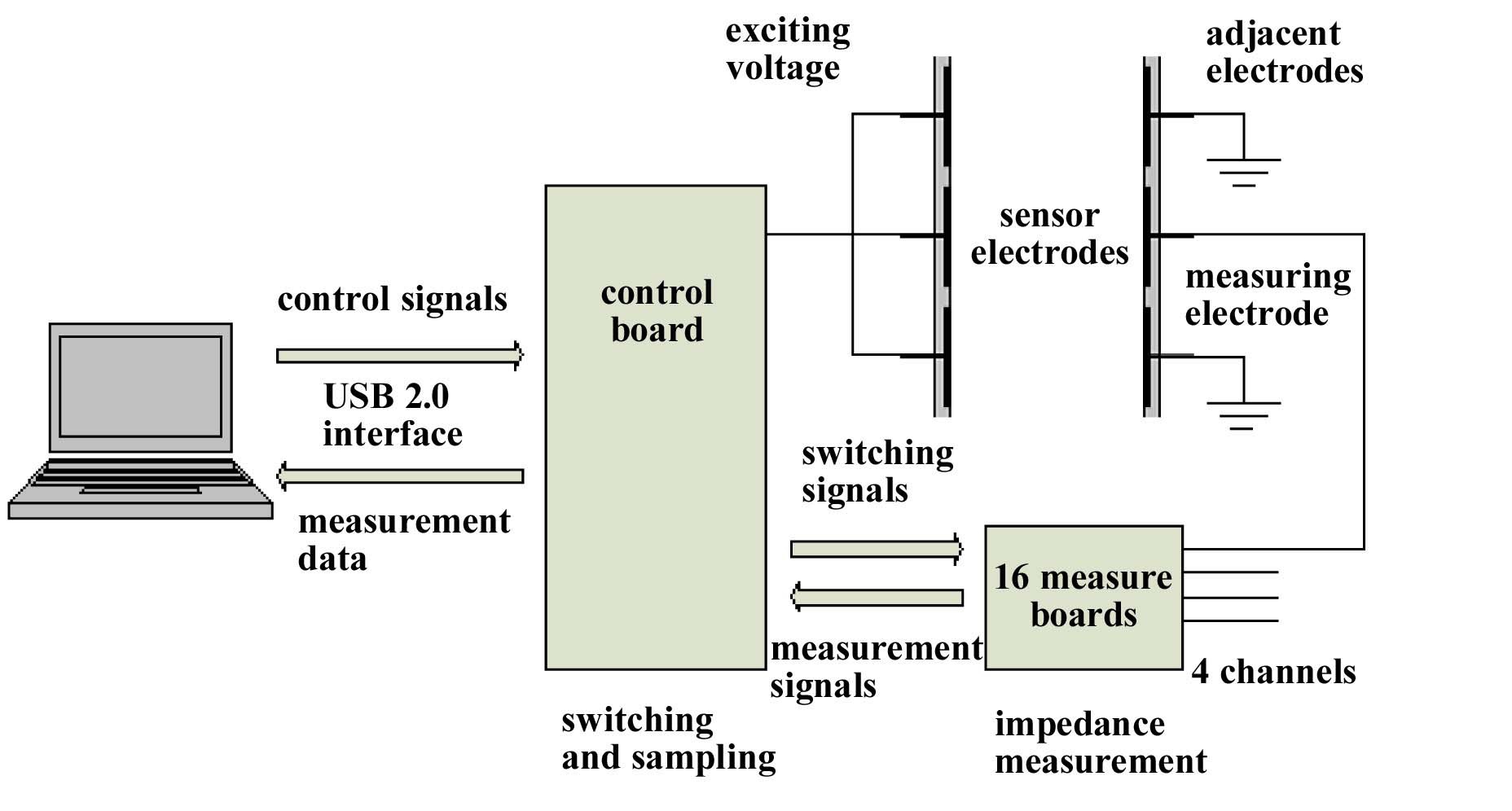
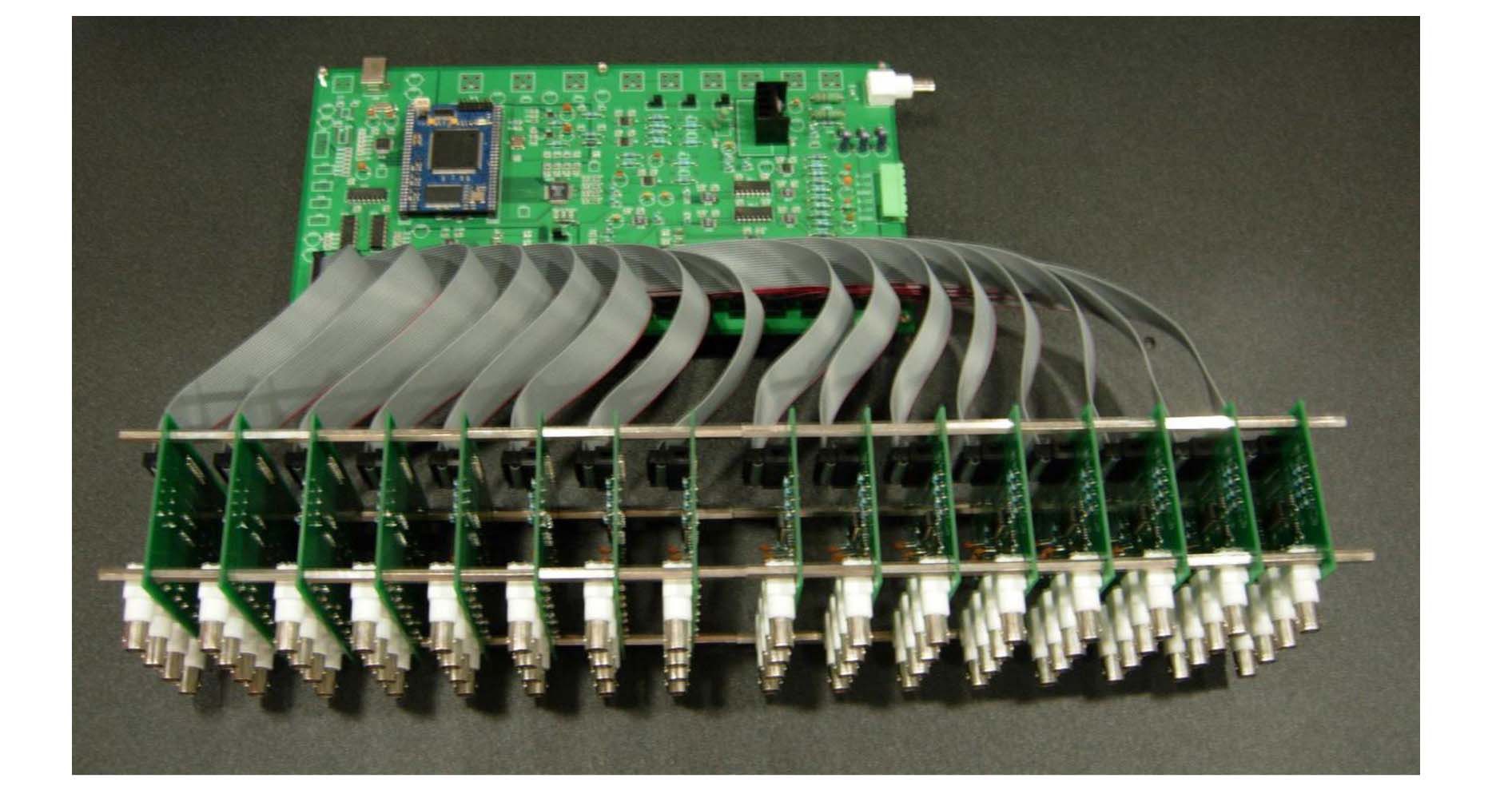
In the present study, a new impedance measuring system was developed. Figure 8 shows a diagram of the impedance measurement system. It consists of a control board and measuring ones. The control board is connected to a computer with a USB 2.0 interface, which can communicate at a maximum speed of 3 MB/sec. When the computer sends a trigger signal to the control board, the control board delivers the measured data at 100 frames/sec to the computer. The control board sends a switching signal to 16 measuring boards, each of which has four measuring channels. The measured impedance signals are delivered to the control board and sequentially to the computer. A total of 64 channels’ data can be measured using the current impedance measuring system. Figure 9 shows a photograph of the coupled control and measuring boards. (Bae et al., 2010)

Since the conductance is proportional to the crosssectional area, the void fraction can be formulated using the conductance ratio of the mixture and water:

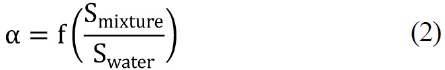
where the conductance of pure water, S_water, is the value at the local point of the test section for flowing water only

as the reference condition. Since the flow conditions of the reference test and two-phase condition are not exactly the same, a compensation process using the impedance of the reference sensor was performed as follows:

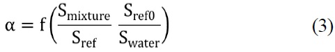
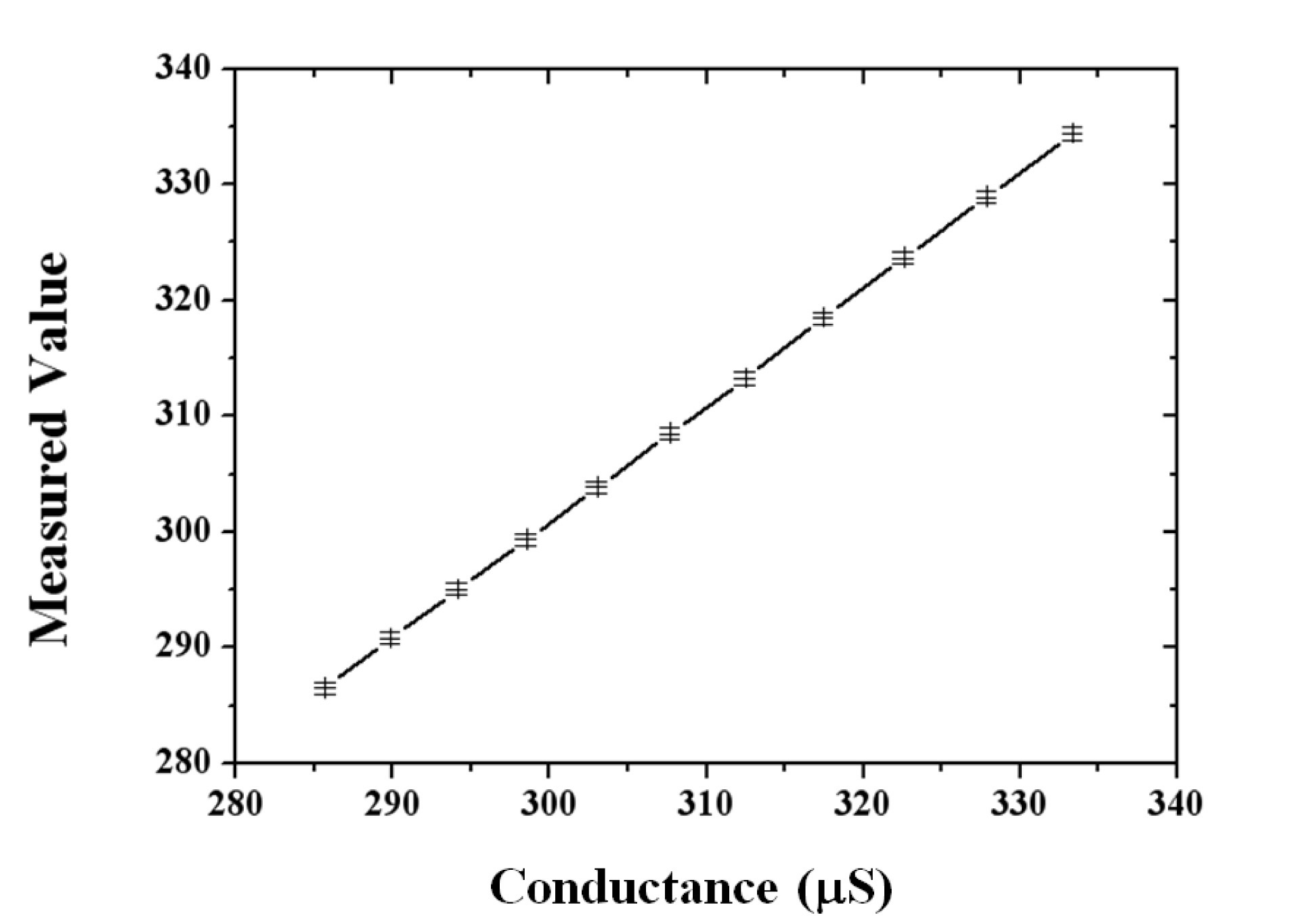
where S_ref and S_ref0 are the conductance measured at the reference sensor for the two-phase condition and pure water flowing conditions, respectively. The impedance measuring system was calibrated using various known resistors. Figure 10 shows very accurate measuring results with less than 0.2% deviation.

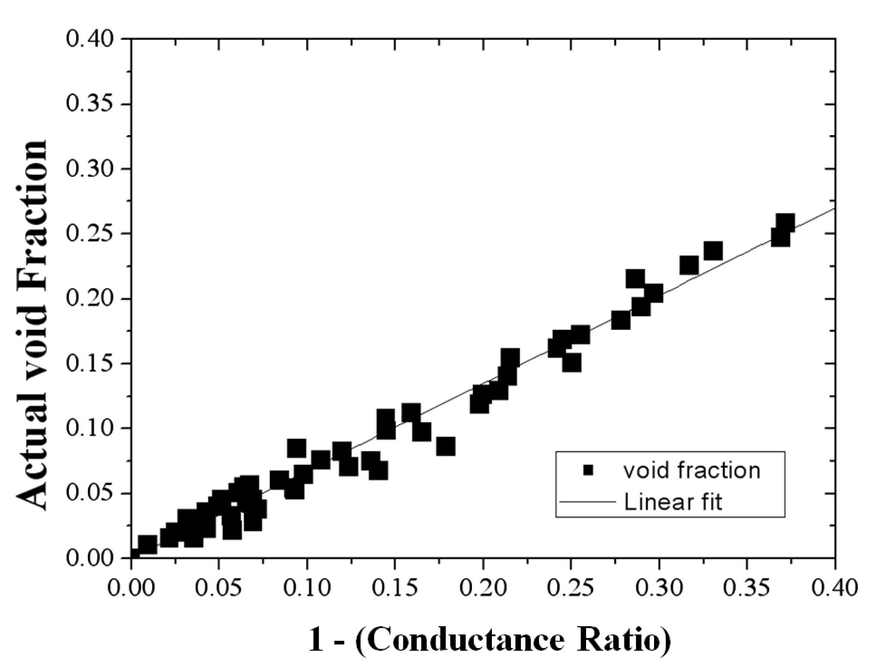
To calibrate the measured impedance value for void fraction data, a calibration was performed using a test section with 4×4 electrodes in the same configuration of electrodes as in the DYNAS system shown in figure 11. Acrylic beads were utilized for the bubble simulators. By controlling the bead configuration, the actual void fraction was analyzed. A conceptual diagram for the calibration

process is shown in figure 12. Figure 13 shows the following relation between the impedance and void fraction:

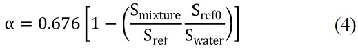
The standard deviation of the above calibrated curve is 1.6%.

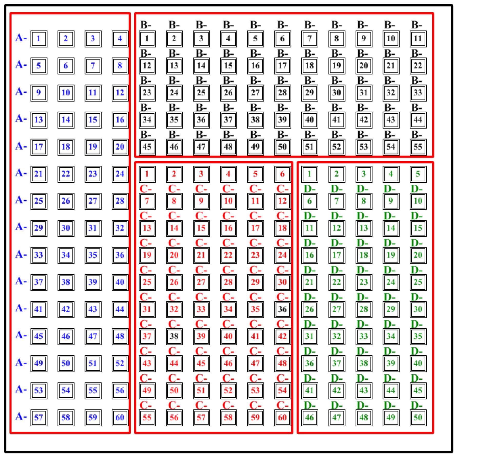
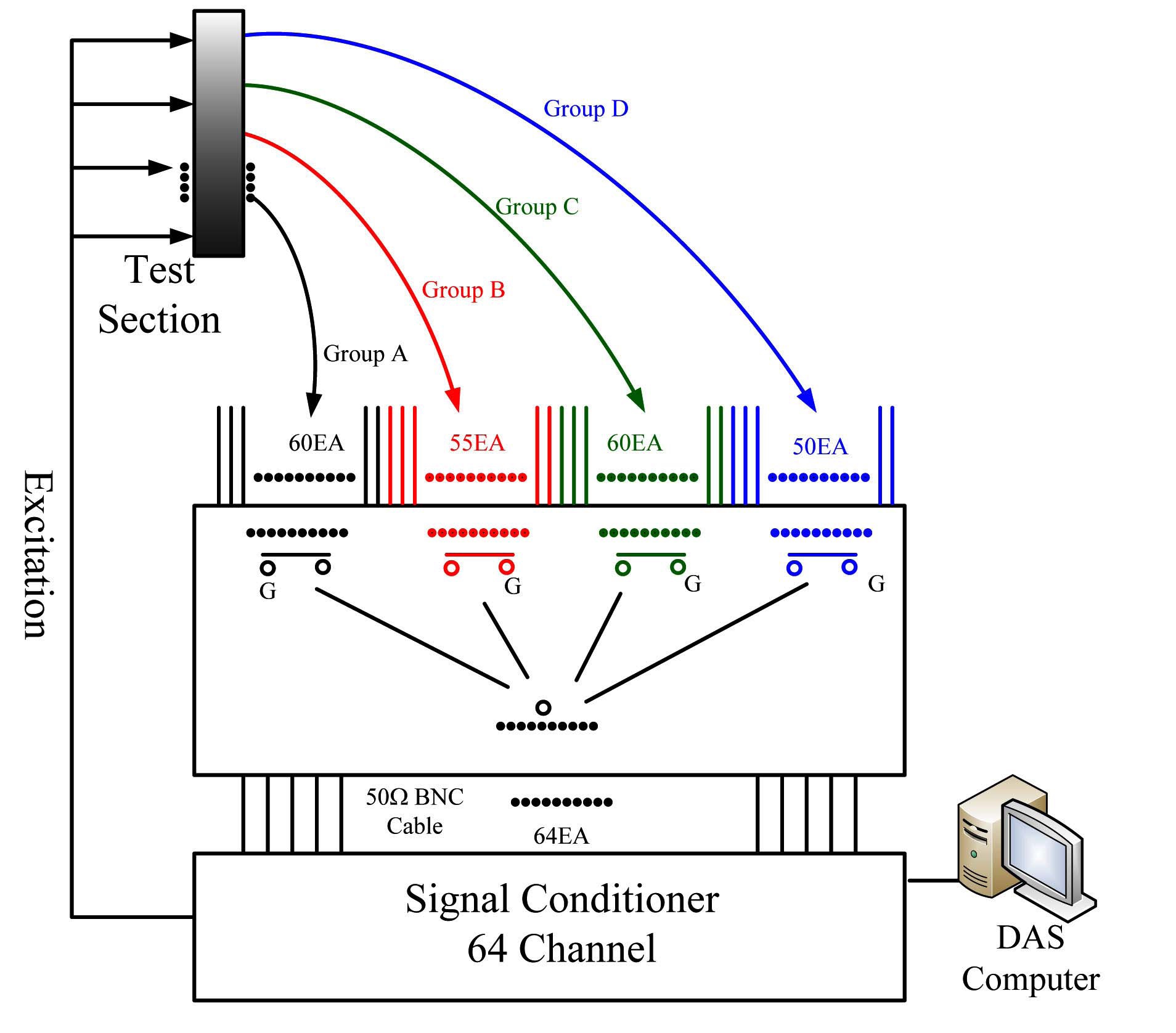
The test section has 15×15 measuring points for a local measurement to obtain a void fraction profile with a sufficiently high resolution. Since the currently developed measuring system has only 64 channels, a switching system was also developed for applying the measuring system with a limited number of channels of DAS for 225 points of local data. By considering the two-phase mixture flow shown in the visualization test, all the local points were grouped into four groups, as shown in figure 14 such that each group of sensing points can contain a long mixture stream. The 64 channel signals can be switched to the specified group channels using relays installed inside the switching block with manual or sequential modes. Figure 15 shows a signal flow diagram for the data acquisition.

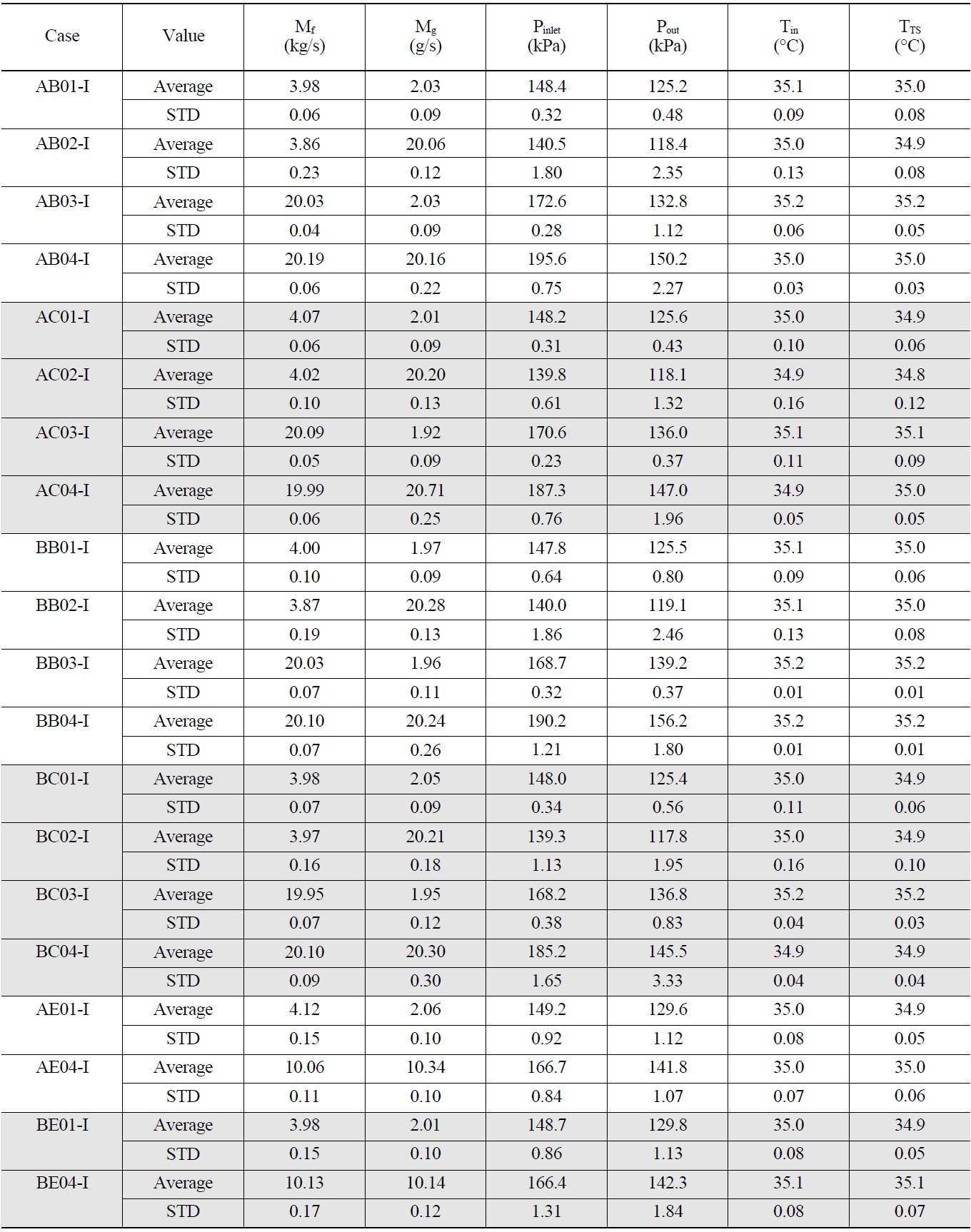
Figure 16 shows the definition of the inlet and outlet nozzles. Each test condition was achieved by selecting an inlet and an outlet nozzle. Table 1 summarizes the averaged values and standard deviations of the measured data of the boundary thermal hydraulic parameters for all test cases.

For the impedance measurement, 20 tests were performed, in which 6 sets of combinations of the inlet and outlet ports were selected. In the present study, 100 seconds of data were acquired at each local point with a 100 Hz/channel sampling speed. The instantaneous measured data were processed for the statistical results

The outlet pressure was not controlled to a specific value. In other words, the pressure value at the outlet nozzle, which is naturally determined under the conditions of the

storage tank water level and desired water/air injection flow rates, was set as a pressure boundary condition. The temperature at the loop and test sections was controlled at 35 ℃ using a heater and cooler imbedded in the storage tank. To obtain data representing various dynamic multidimensional two-phase movements, combinations of maximum and minimum water and air flows were applied. For each selected inlet and outlet nozzle combination, the water flow ranged from 2 to 20 kg/s, and the air flow rate ranged from 2.0 to 20 g/s, which corresponds to 0.4 to 4 m/s and 0.2 to 2.3 m/s of superficial liquid and gas velocities based on the inlet port area, respectively.

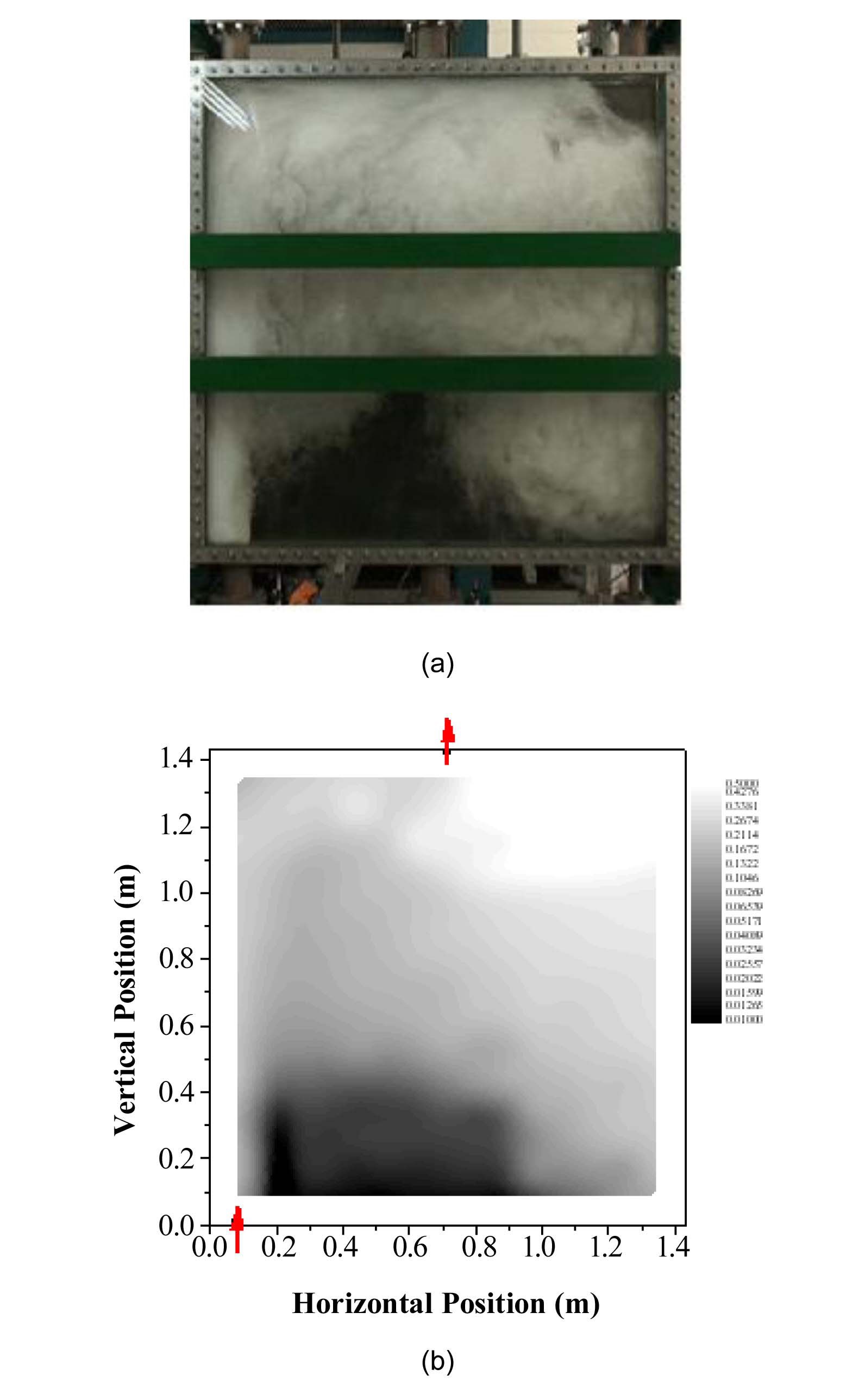
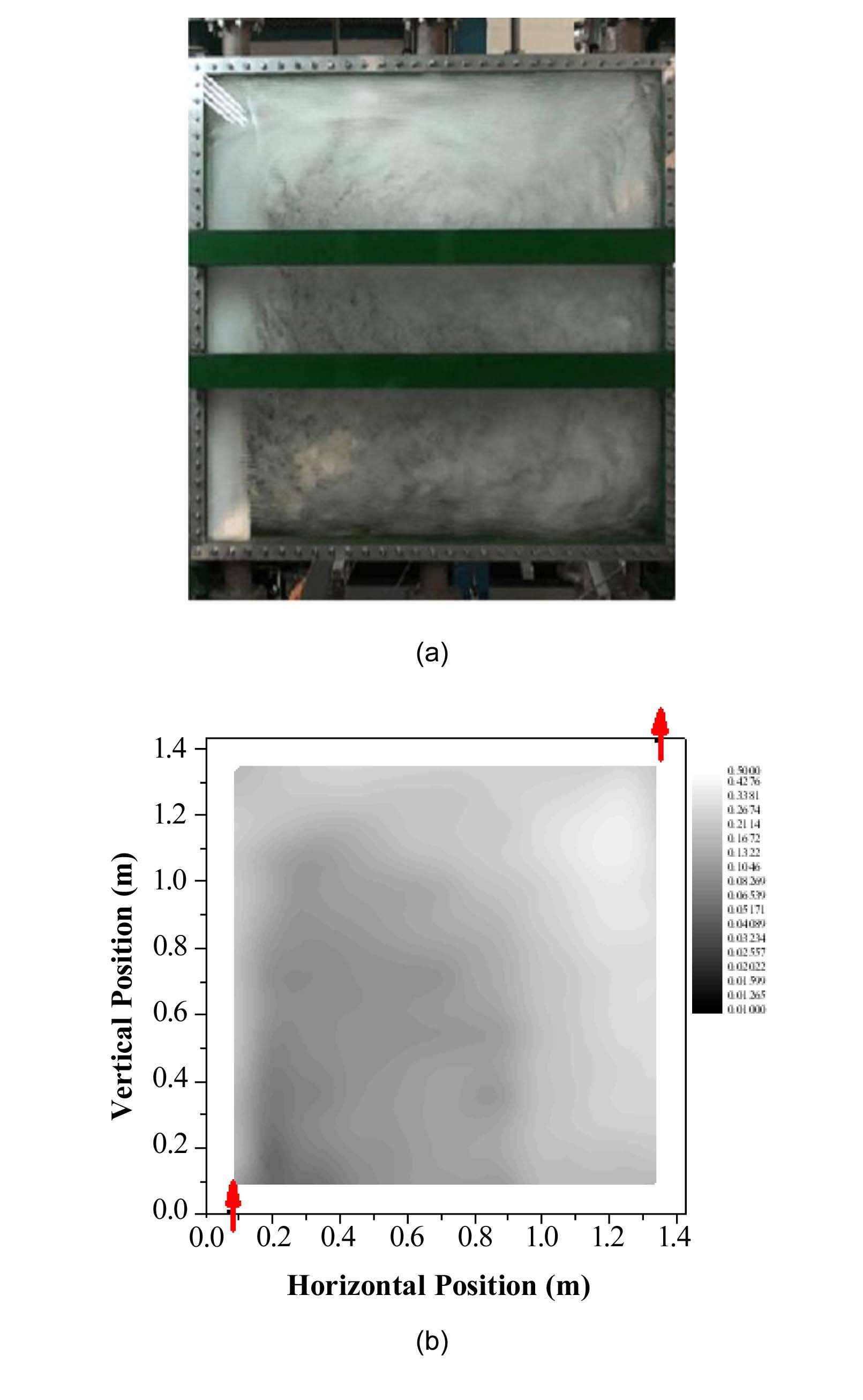
In the present paper, three typical test results were presented. Figure 17 shows the results for combinations of inlet A and outlet B for high water and air flow conditions, AB04. The measured impedance at each point was converted to void fraction data using a calibration curve and plotted into a 2D contour form, which were compared directly with

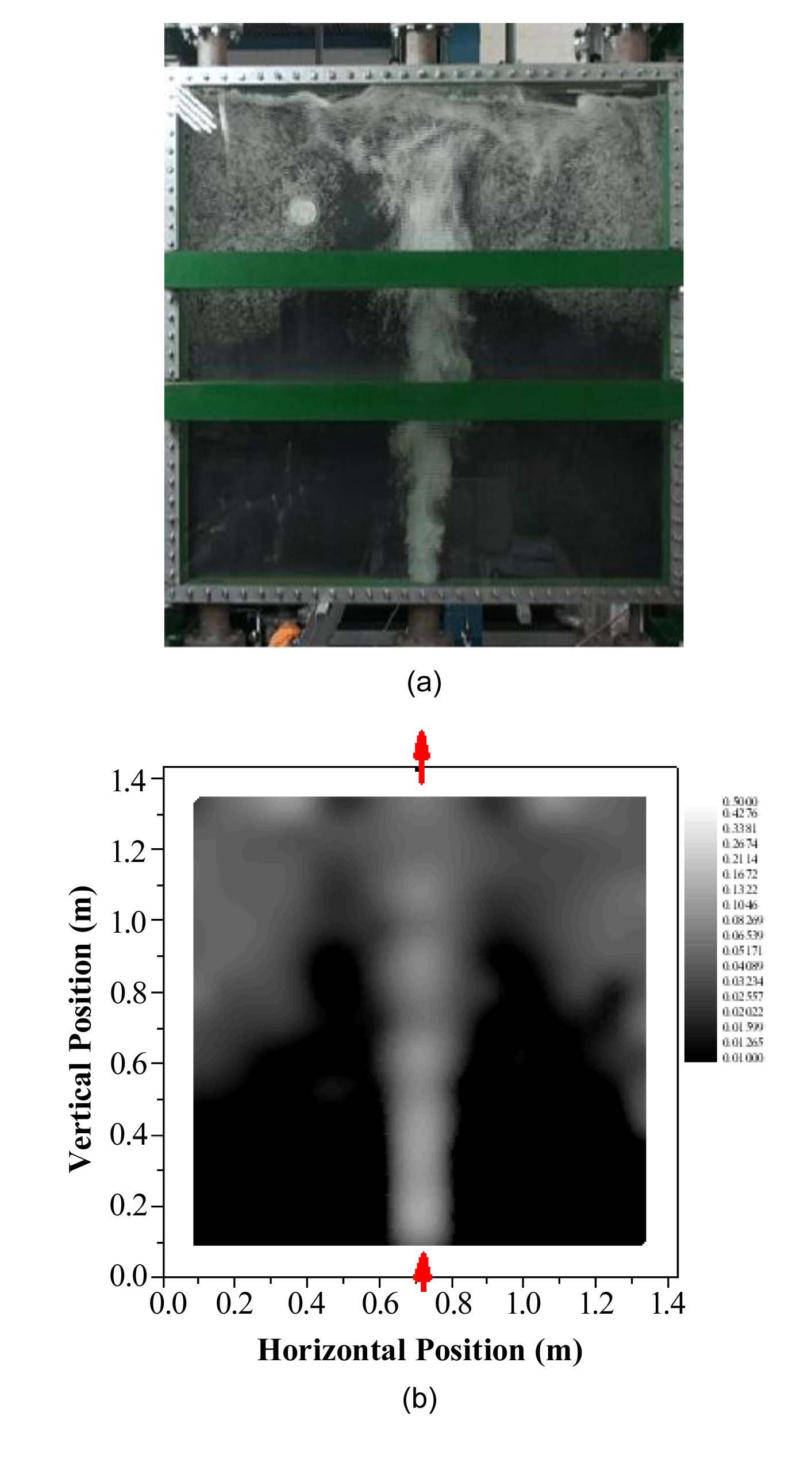
the visualization results. A highly strong upward flow was formed near the left wall and discharged at the central top nozzle after flowing across the upper part of the test section. Owing to the extreme momentum inertia, the two-phase mixture passing the outlet nozzle moved toward the upper right wall and flowed downward at the right side of the test section, which shows a rotated flow pattern. A stagnant air pocket is formed in the upper right region. The void profile from the impedance measurement reflected the visualization results well. Figure 17(b) shows a straight stream near the left wall and accumulation of air toward the upper right part, which is very similar with the visualization. Figure 18 shows the void profile for cases in which inlet A and outlet C were selected with high water and air flow conditions, AC04. Figure 19 is for inlet B and outlet B with low water and air flow rates. The measured void profiles are very plausible when compared with the visualization images. To check the accuracy of the measured data in

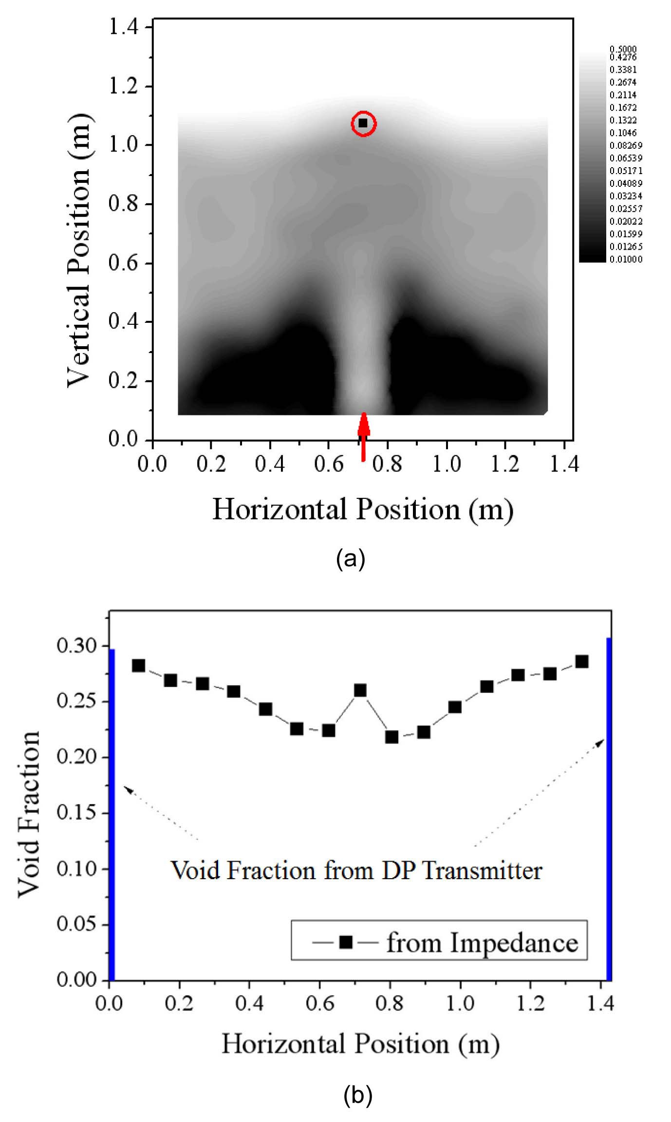
another way, the liquid levels near the two side walls measured from the differential pressure transmitters were compared with those from the impedance measurement. The AE and BE combinations, where a free surface is formed at the level of the outlet nozzle on the face of the slab wall, were selected for comparison. Since the cases do not inflict a dynamic pressure force on the hole at the side wall for the pressure measurement, the measured differential pressure is come from the hydro-static head. For the other cases which have outlet nozzles at the top of the test section, more or less dynamic pressure components can be incorporated into the measured pressure at the side wall. In the current study, three data points measured at both the side wall at BE04 case and the right wall at AE04 case, which have a meaningful void fraction level, were

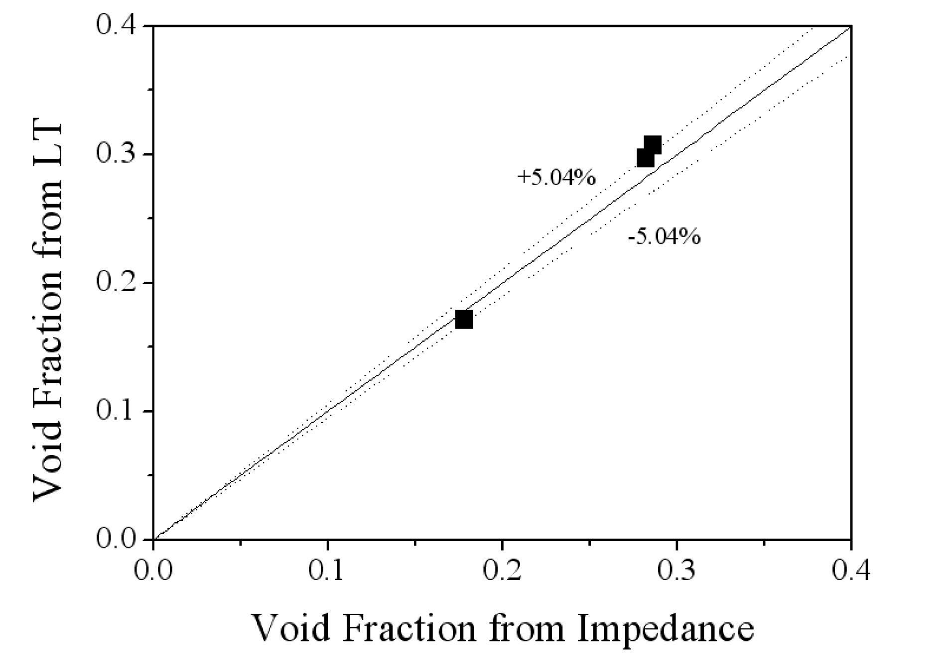
considered for comparison. Figure 20(a) shows the contour of the void fractions from the impedance measurements. The average void fraction profile along the lateral axis was plotted in figure 20(b), which was obtained by averaging the void fractions from sensors on the same vertical line. The two liquid levels measured by the differential pressure at each side wall are expressed as bars on the side of the plot in figure 20(b). A peak void fraction was measured at the laterally central position owing to the major air flow stream. After a reduced void region out of the stream, the void fraction is increased again toward the side walls, which shows a symmetric void profile. As shown in the figure, the two measured void fractions near the wall from the impedance method and differential pressure measurement agree well with each other. Figure 21 shows a 5% deviation between the two measured average void fractions.

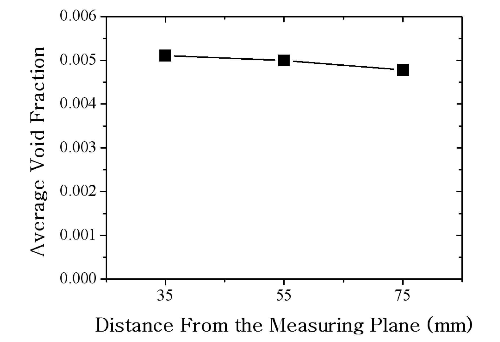
The uncertainty components were considered for (1) the void fraction calibration curve, (2) the effect of the gap distribution of the void fraction, and (3) the temperature effect. The effect of the gap void profile was evaluated using an electric field analysis. The bubble path was set at 3×15 local points between slabs in the plan view as shown in figure 22. The void fractions of each 15 columns were averaged. The three average void fractions were

analyzed by averaging the void fractions at 15 columns on each plane at 35, 55 and 75 mm in the gap direction. For the analysis, a 40 mm spherical particle was used for the bubble representation. Figure 23 shows the average void fraction at each plane, which has less than a 10% deviation. By referring to the analysis, the measured impedance data representing the local average void fractions between the two slabs were assumed to have a maximum of 10% uncertainty owing to the gap void distribution.

The conductance increases with the temperature. Through a preliminary test, the variation of the conductance was measured as 9.88E-6 S/℃. In this test, the maximum deviation of the temperature was controlled to within 0.3 ℃. Using this information, the variation of the void fraction owing to the temperature variation of 0.3 ℃ is 0.4%, as an absolute void fraction value. By considering 1.6% of uncertainty induced by the calibration curve, the relative bias error is analyzed as 10.9% for the case of 10% void fraction data. For 30% void fraction conditions, the relative uncertainty is analyzed as 10.2% of measured value. The above analysis can be expressed as follows:

where

Ub,tot : total bias error

Ub,gap : Bias contributed from phase distribution across gap direction (10% of average void fraction)

Ub,Temp: Bias contributed from temperature (0.4% in absolute void fraction)

Ub,Cal : Bias contributed from calibration curve (1.6% of average void fraction)

For 10% void fraction as an example,

which is 10.9% of the average void fraction.

The precision errors were measured within the range of 3% to 4% for the overall void fraction level.

To identify and generate experimental data for a twodimensional two-phase flow, experiments were performed using a large-scale slab type test section called DYNAS. The local void fraction profile database measured in the current 1.43 m×1.43 m scale was considered as very useful for the system code validation since the amount of literature data is very limited. To achieve the desired data set, an impedance measuring system was uniquely developed including appropriate calibration process and multiplex data acquisition for numerous measuring points.

Various patterns of multi-dimensional two-phase flow could be obtained by selecting different combinations of inlet and outlet nozzles of the test section. A set of local void fraction data were acquired by 225 sensors on the slab using an impedance measurement system, as well as boundary thermal hydraulic parameters. The measured void fraction was also analyzed with consideration of the key components for the uncertainty embedded in temperature variation, local phase distribution, and calibration curve. The obtained void fraction profiles from the impedance measurement were compared with the images from a CCD camera, and were found to be very plausible. The experimental data will be utilized to validate the thermal hydraulic models and correlations of a nuclear system analysis code.

α Void fraction [-]

Db,max Maximum allowable bubble size [m]

g gravitational acceleration [m/s2]

S Conductance [1/Ω]

Δρ Density difference between gas and liquid [kg/m3]

σ Surface Tension [N/m]