The ionosphere influences every user that uses navigation signals, and is the largest error in signal transmission processes. When signals from navigation satellites pass the ionosphere, the navigation signals experience refraction, reflection, and attenuation by the total electron content (TEC) of the ionosphere.

A global positioning system (GPS) reference station network, which is distributed globally or locally, plays an important role in the precise calculation of ionospheric TEC (Skone 1998, Fedrizzi et al. 2005). Especially, with the development of information and communication technology and the Internet, GPS data can be received in real time from a remote location. The data obtained in real time is widely used for real-time ionosphere studies as well as highprecision positioning (Mannucci et al. 1998, Gao & Liu 2002).

Studies on the analysis of the ionospheric characteristics are essential for precise positioning of users. In general, single-frequency GPS users utilize the Klobuchar model to estimate ionospheric delay error (Klobuchar 1987). On average, this model can correct ionospheric delay error by up to about 50% (Komjathy 1997). As the error from the ionosphere cannot be completely removed, single-frequency GPS users are not capable of precise positioning. In addition, the ionospheric TEC disturbance caused by increased solar activity and geomagnetic storms has large effects on navigation signals such as signal interruption or the increase in error. Ionosphere studies using GPS are also used to analyze the characteristics of earthquakes (Heki 2011, Artru et al. 2005). In the case of the 2010 Chile Earthquake (February 2010) and the Great East Japan Earthquake (March 2011), enormous energy was generated from the earthquake epicenter, and was transmitted to the atmosphere. Waves transmitted to the upper atmosphere in various forms affect ionospheric TEC, and thus the characteristics of the wave forms generated by earthquakes (e.g., Rayleigh surface wave and tsunami wave) could be analyzed. Therefore, the intensity or characteristics of earthquakes could be examined through the detection of the variation of TEC.

Recently, studies have been conducted to detect the variation of the ionosphere quickly and minutely (Spogli et al. 2009, Prikryl et al. 2013). Especially, Prikryl et al. (2013) used 1 Hz and 50 Hz GPS data to detect the variation of TEC caused by geomagnetic storms at high latitudes. They observed scintillation, and also performed verification research using the radar and ionosonde observation data.

Blewitt et al. (2009) emphasized the use of 1 Hz GPS data for real-time crustal deformation monitoring and tsunami warning, which are caused by earthquakes. Also, Komjathy et al. (2012) showed that it is possible to monitor the variation of ionospheric TEC caused by earthquakes using a realtime GPS observation network, which is distributed globally. This indicates that the future research on and demand for ionospheric TEC are focused on real-time monitoring.

In this study, the strategies for the real-time monitoring of ionospheric vertical TEC (VTEC) are introduced, and the calculation results of ionospheric VTEC values during 1 hour are presented, which use the 1 Hz data from the nine global navigation satellite system (GNSS) reference stations operated by the Korea Astronomy and Space Science Institute. In addition, the time series of the variation of VTEC values is also provided.

To estimate ionospheric TEC precisely, the use of dual frequency GPS observation data (L1~1575.42 MHz and L2~1227.60 MHz) is essential. The receivers of GNSS reference stations, which are fixed on the ground, receive and store the GPS observation data that consists of code and carrier phase. The methods for calculating TEC using GPS observation data have been introduced in detail in a number of papers (Calais & Minster 1998, Mannucci et al. 1999, Davis & Hartmann 1997, Afraimovich et al. 2001, Otsuka et al. 2002). When GPS navigation signals pass through the ionosphere, signal delay occurs due to the free electrons in the ionosphere. This delay can be easily calculated using Eq. (1) (Sardon et al. 1994).

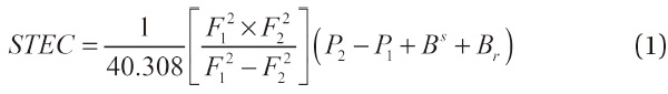
where P_i(i=1,2) is the observed pseudorange value, and F_i(i=1,2) is the GPS signal frequency. B^s and B_r represent the differential code bias (DCB) of the satellite and the receiver DCB, respectively. STEC represents the ionospheric TEC in the line-of-sight direction, and this value is converted to VTEC using an appropriate mapping function. Also, in this study, a carrier phase smoothing method, which uses both code and carrier phase, was utilized to increase the accuracy of TEC (Kleusberg 1986).

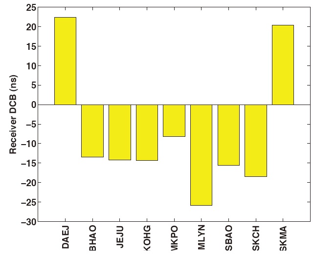
DCB is the largest error in calculating ionospheric TEC with the use of observed dual frequency GPS values. Moreover, several GPS receivers have a DCB value of dozens of nanoseconds (ns), and this should be calculated for an accurate TEC calculation (Choi et al. 2011). If the DCB value is not accurately compensated, the reliability of the estimated TEC value would decrease. In this study, the DCB values calculated in advance (i.e., the day before) were applied to the real-time TEC calculation. Fig. 1 shows the estimation of the receiver DCB values for the nine GNSS reference stations operated by the Korea Astronomy and Space Science Institute, which were estimated in advance for the TEC calculation. The Daejeon (DAEJ) and Seoul (SKMA) GNSS reference station receivers (Trimble NetRS) had a DCB value of more than 20 ns, and the other GNSS reference station receivers (Trimble NetR9) had a minus (-) value. Especially, the Milyang (MLYN) reference station receiver had a large DCB value (about ？26 ns), which could have a large effect on the TEC calculation.

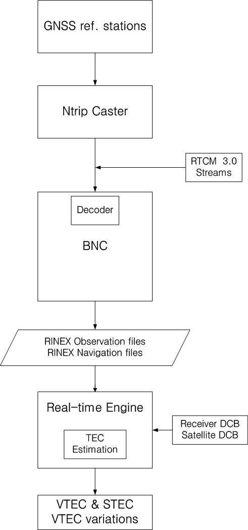
Fig. 2 shows the flow chart of the data processing for the real-time TEC calculation. The nine GNSS reference stations operated by the Korea Astronomy and Space Science Institute are evenly distributed over the Korean peninsula. Some of them are connected with the data center in Daejeon via the Internet network, and the others are connected with the data center in Daejeon via the dedicated lines. The GNSS reference stations receive the GPS signals in real time, and transmit the raw data (binary type) to the data center. The raw data followed the Radio Technical Commission for Maritime Service (RTCM) 3.0 data transfer standard protocol, and the Networked Transport of RTCM via Internet Protocol (NTRIP)

caster was used to control the transfer and flow of the GNSS data on the Internet.

As the RTCM data transmitted from NTRIP is raw data and is encoded, the decoding and conversion of this information are required. In this study, the BKG Ntrip Client (BNC) software version 2.7 developed by the Federal Agency for Cartography and Geodesy (BKG) in Germany was used. The BNC software examines the quality of GNSS data, and performs the conversion of raw data to Receiver Independent EXchange Format (RINEX) so that users can easily understand. Thus, the most basic form of data for the TEC calculation can be obtained using the BNC software. If the BNC software is not available, users can calculate TEC by directly converting the RTCM information that is transmitted

to NTRIP. In this case, the RTCM information received at each port needs to be checked continuously, and the data needs to be converted and stored in a separate buffer.

The RINEX file was generated at an interval of 300 seconds, and the data was stored every second. In other words, the TEC values were calculated every 300 seconds, and TEC was calculated at each observation time. If the data from nine GNSS reference stations is used and every reference station receives 10 GPS satellite signals, the total number of TECs, which are to be calculated every 5 minutes, is 27,000=(=9×10×300). The information that is acquired at the end includes the TEC values in the vertical direction and the line-of-sight direction, and the variation of TEC depending on time. Especially, a real-time ionospheric TEC monitoring study focuses on the variation of TEC values rather than the TEC values themselves.

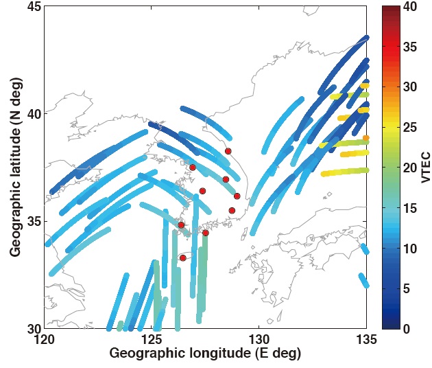
To obtain ionospheric TEC values over the Korean peninsula and monitor the variation, the GPS observation data received at the GNSS reference stations on January 1, 2013 was used. The raw data from the nine GNSS reference stations was transmitted to the data center every second, and the RINEX file, which includes the 1 Hz observation data, was generated at an interval of 5 minutes at the data center. Using this GPS observation data from the nine GNSS reference stations that was stored every 5 minutes, the TEC values over the Korean peninsula during 1 hour were obtained as shown in Fig. 3. The data processing period was from 0:00 UT (09:00 KST) to 1:00 UT (10:00 KST). Fig. 3 shows the obtained variation of the VTEC values depending on the ionospheric pierce point (IPP) of the GPS navigation signals. Also, the small dots represent the position of the GNSS reference stations.

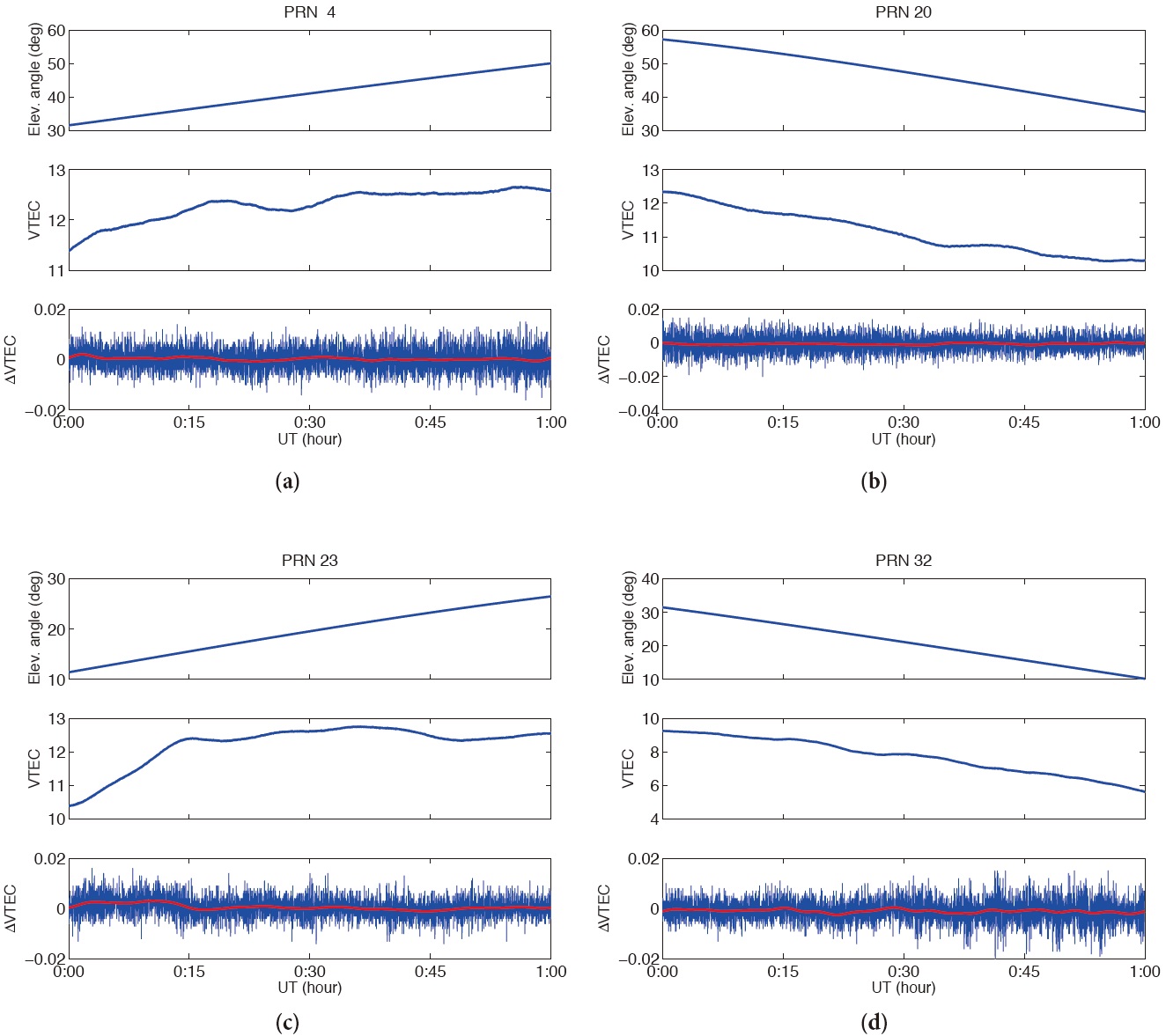
To minutely analyze the VTEC values estimated using the GPS observation data, the change in the elevation angle of satellites, the VTEC values, and the variation of the VTEC values depending on time were obtained for each GPS satellite. Figs. 4a-4d show the data processing results of the GPS satellite pseudo random noise (PRN) 4, 20, 23, and 32, respectively. For the satellite PRN 4, the elevation angle increased by about 18 degrees from 32 degrees to 50 degrees, and the VTEC value increased by 1 TEC unit (TECU) in the

first 20 minutes (1 TECU is 10¹⁶ electrons/m², which indicates that there are 10¹⁶ free electrons per square meter). Then the value remained stable during the next 40 minutes without a large variation. Also, the variation of the VTEC values (i.e., (VTEC_n+1-VTEC_n)/1sec) was ±0.01 TECU. In other words, the time variation of the VTEC values was insignificant, and ΣK_p, the geomagnetic index for this day, was 0+, which indicates that the geomagnetic activity itself was very stable. The Dst index was also found to be very stable using the data from the website of the world geomagnetic data center (http://wdc.kugi.kyoto-u.ac.jp/dst_realtime/201301/index.html).

Fig. 4b shows the information on the elevation angle and the VTEC value of the satellite PRN 20. A notable point is that the variation range of the VTEC values depending on time decreased although the elevation angle of the satellite decreased. This is thought to be related with the signal-tonoise ratio of the GPS signals received at the GNSS receivers, but more detailed research (e.g., performance analysis of the receivers) is needed to find the cause. Fig. 4c shows the obtained information of the satellite PRN 23, which is similar to the result of the satellite PRN 4 in Fig. 4a. After the data processing, slight changes in the VTEC values depending on time were observed within 15 minutes. This is thought to be because the increased observation noise affected the variation of the VTEC values since the elevation angle of the satellite was less than 15 degrees.

Fig. 4d shows the data processing result of the satellite PRN 32. The elevation angle of the satellite decreased from 32 degrees to 10 degrees during 1 hour, and the VTEC value also decreased by more than 3 TECU. For the variation of the VTEC values of the satellite PRN 32 depending on time, the variation range of ΔVTEC values increased as the elevation angle decreased.

When the elevation angle of a GPS satellite is low, it generally takes more time for the navigation signals transmitted from the satellite to pass the ionosphere, which increases the error or the observation noise. The results in Figs. 4c and 4d support the above-mentioned explanation. However, the result in Figure 4b is inconsistent with the above explanation, and there can be various causes for this inconsistency. It could be due to the characteristics of the GPS signal-to-noise ratio at a specific elevation, or the problem of the receiver hardware performance. Alternatively, it could be because the elevation angle of the satellite PRN 20 was maintained above 25 degrees during the data processing period, whereas the satellite PRN 23 and the satellite PRN 32 had a lower elevation angle. This needs to be addressed carefully since the characteristics could differ depending on GNSS receivers or satellite signals.

In this study, a real-time ionospheric TEC monitoring study was performed using the data from the nine GNSS reference stations operated by the Korea Astronomy and Space Science Institute. The data processing was carried out by converting the 1 Hz raw data, which is transmitted from each GNSS reference station, to RINEX every 5 minutes. The data processing period was 1 hour, and the elevation angle of satellites, the VTEC values, and the variation of the VTEC values were obtained for each GPS satellite PRN. The analysis indicated that the ionospheric VTEC values over the Korean peninsula did not show a large variation, and the variation of the VTEC values depending on time was also stable. However, for the satellite PRN 20, the variation of the VTEC values depending on elevation angles showed a trend that is different from other satellite signals. As this phenomenon is related with the observation noise of the GPS signals, further research is thought to be needed.

In this study, the research method for a real-time ionospheric TEC monitoring study was presented. Also, the VTEC values and the variation of the VTEC values depending on time were calculated and analyzed. These results are expected to be useful for the fields that utilize ionospheric TEC values in real time.