The Optical Wide-field Patrol (OWL) network is a project designed for the surveillance of space objects such as artificial satellites, rocket bodies and their debris, which can threaten a country’s space & ground properties, as well as human life. To achieve this surveillance, multiple optical telescopes will be built all around the world. These telescopes are small (0.5 m in aperture), operated automatically, and controlled by staff in a single headquarter. The observation images from these telescopes must be reduced quickly and automatically, and sent to the headquarter daily. The image reduction procedure of OWL should include detection of bright sources from the images, identification and separation of traces of moving objects from them, determination of physical & positional parameters of the detected moving object, and finally, combining with the time log data. As such, the development of a reduction algorithm that can be operated on the remote sites is essential. In this paper, the steps of developing the reduction algorithm and the results are presented.
In Section 2, the OWL testbed and its hardware will be introduced. In Section 3, the test observation at the testbed will be described. In Section 4, the details of the reduction algorithm will be explained. In Section 5, the results and their discussion will be presented, and finally Section 6 provides a summary.
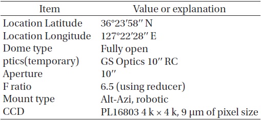
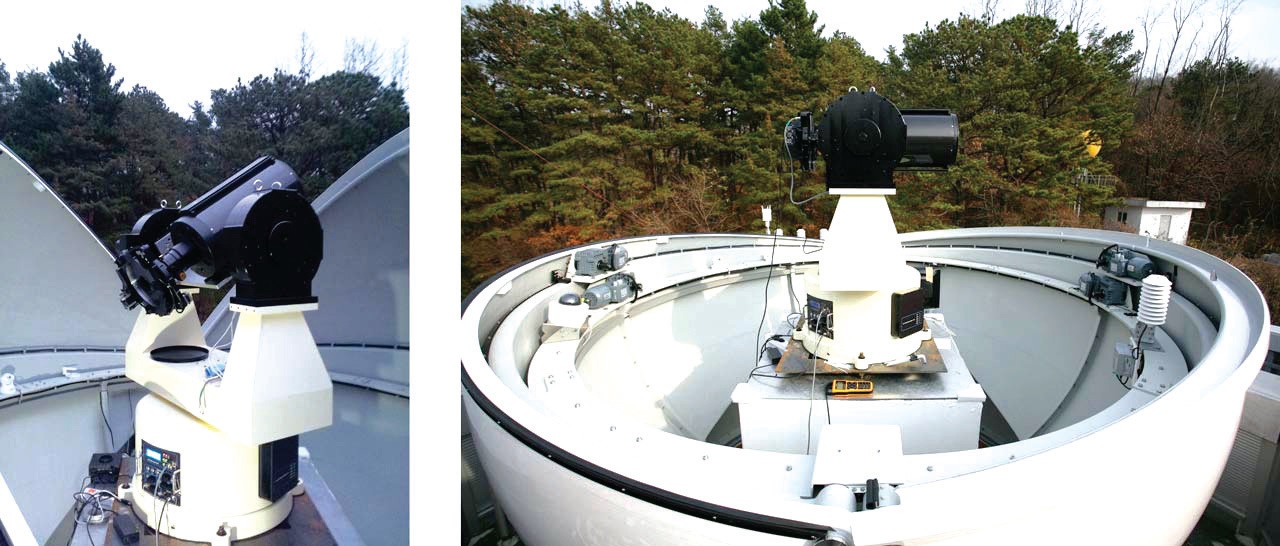
The prototype of the OWL station (OWL testbed) is located at Korean Astronomy and Space Science Institute in Daejeon, Korea. The dome can be fully opened and the mount can move quickly for rapid surveillance of the whole sky. A commercial GS Optics 10′′ telescope is temporarily used for test and development purpose (Table 1 and Fig. 1).
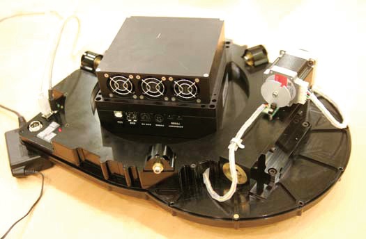
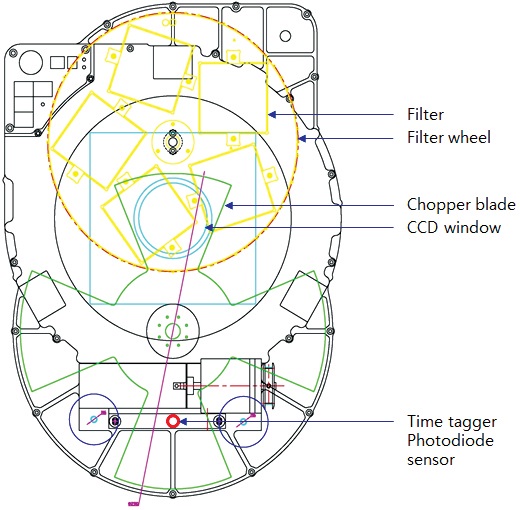
The OWL Detector Subsystem (DT system) is composed of a CCD camera, a filter wheel, a chopper and a time tagger. Each part is explained in the following:
i. Filter Wheel. The OWL filter wheel holds 4 filters of B, V, and C (Clear).
ii. CCD Camera. Finger Lake Instrument PL16803 CCD camera is selected for OWL image acquisition. The
[Table 1.] OWL testbed specifications.

OWL testbed specifications.
sensor chip is a Kodak KAF-16803 Full Frame Front Illuminated Sensor with a 4096×4096 array of 9μm-sized pixels. Gain is 1.43 in e-/ADU and readout noise is 8.23 in e-.
iii. Chopper. The chopper is used to cut the trail of a moving object on the image into multiple streaks. It has 4 rotating blades which intersect the light rays from the target into the CCD. Before every CCD exposure, the chopper waits at its home position and starts to rotate just after the shutter is open.
iv. Time Tagger. The chopper open/close status is recorded with the time using the time tagger. The time tagger is composed of a reflective sensor, or a photodiode, connected via RS232 serial line to a small box which encloses a simple micro processor. This
processor records the timestamps of chopper open/close situations detected by the photodiode, and transfers the log record data via USB - to - serial line to the OWL DT server.

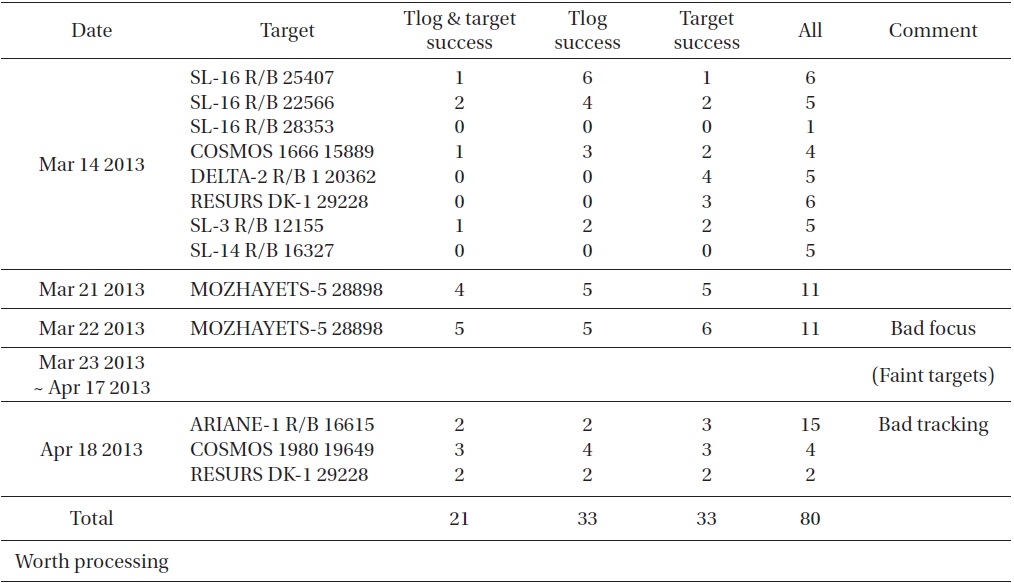
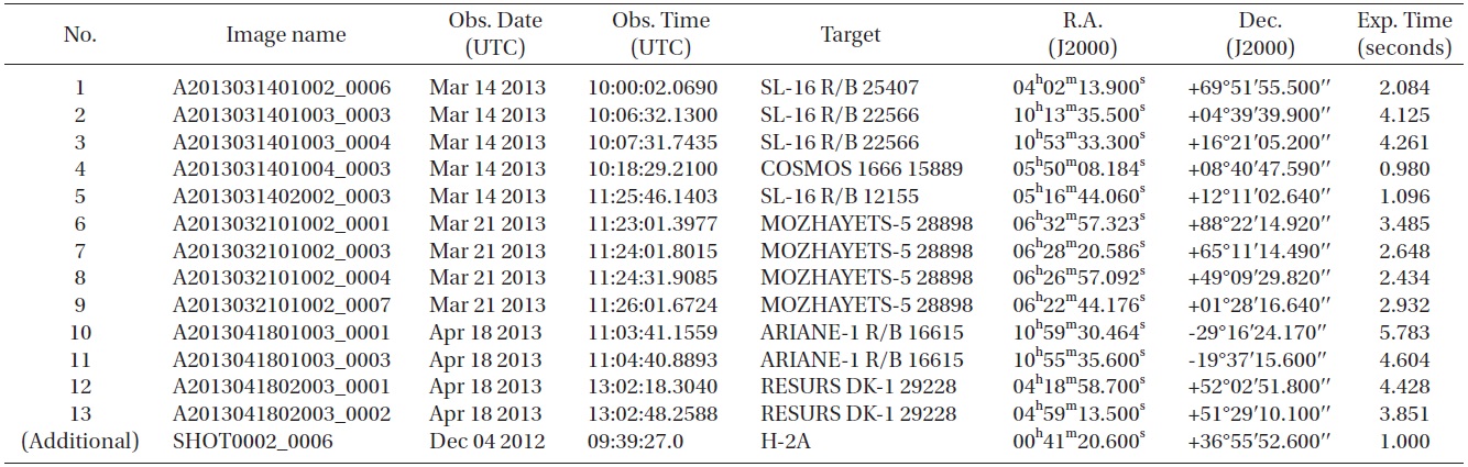
OWL test observation summary. “Date” is the UTC date of the observation, “Target” is the name of the target object (most of them are debris of rocket body - denoted by ‘R/B’ - or artificial satellites with NORAD number), and “Tlog & target success” is the number of successful time tagging log acquisition & target pointed in the CCD frame.
Fig. 2 shows the OWL detector subsystem (DT system) hardware, and Fig. 3 provides the design of the DT system.
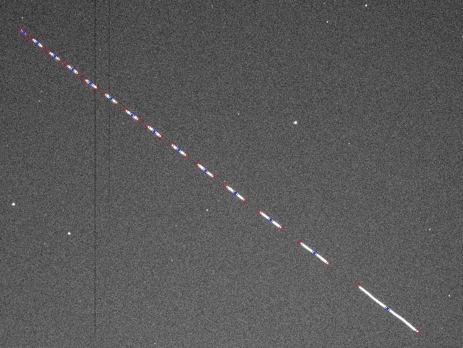
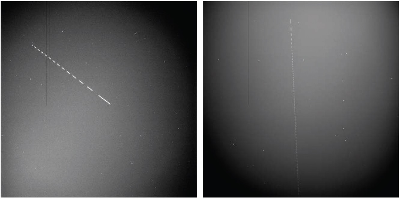
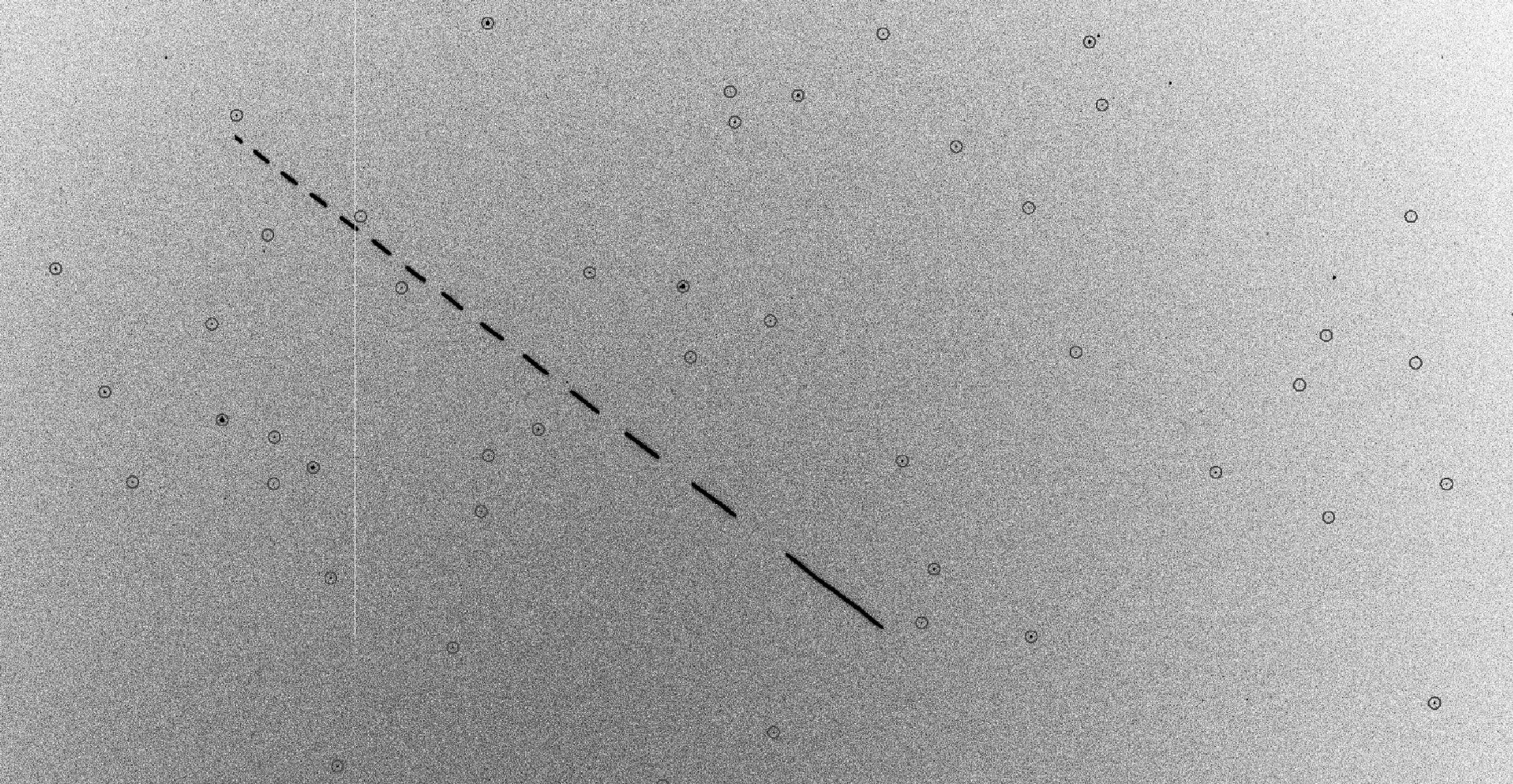
Using the OWL testbed, we performed test observations during a period of about one month from March to April of 2013. Table 2 provides a summary of the observations. As can be seen in Table 2, not all of the trials were particularly successful because of bad weather, focus or tracking failure, unstable time tagger status, targets being too faint and other factors. From the total of 21 successful images, 13 final images were selected for the development of the reduction pipeline via visual inspection after excluding target images that were cloudy or too faint (Table 3). The additional 14th image, SHOT0002_0006, is included because it provides a good example of streaks. Fig. 4 shows examples of OWL test observation images.
Just after the CCD shutter is opened, the chopper starts to rotate from the home position. At the home position, the chopper is aligned so that the CCD window is open between the blades. During the exposure, the CCD window is obscured (closed) and opened in turn, repeatedly. The reflective sensor (photodiode), placed at the opposite
[Table 3.] List of test observation images for reduction algorithm development.

List of test observation images for reduction algorithm development.
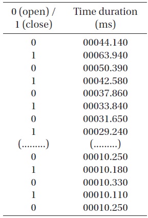
side of the wheel station to the CCD window, detects this situation and records it with the time durations of every open or closed state. If the CCD window is “open”, the state is denoted as “0”, and “closed” is “1”. Table 4 shows a sample time tagging log record. The first column is the open/closed state and the second is the time duration of the state, in milliseconds. Because the chopper starts from a stationary condition and accelerates to rotate, the time durations at the beginning part of the record are relatively large and become smaller as time goes on, until they settle at a constant value. Using this nature of acceleration, the direction of streaks of a moving object can be identified.
4.1 Streak detection using SExtractor
Streak detection is a specific procedure of OWL image reduction. The goal is to detect line-shaped objects from a CCD image and characterize their geometrical parameters. There are several suggestions for streak detection (Montojo et al. 2011, Levesque & Buteau 2007). But here, we adopted an open source photometry software package, SExtractor (Bertin & Arnouts 1996). SExtractor is very quick, easy-to-operate photometry software that can be used for finding
[Table 4.] A sample time log data.

A sample time log data.
sources brighter than a user-specified noise level over the sky background. It gives high precision X &Y pixel coordinate values of the source position, roughly estimated magnitude and its error, and notably, various “shape parameters” (Bertin 2006).
The output parameters from SExtractor (Bertin 2006) used in OWL image reduction are as follows:
i. X_IMAGE & Y_IMAGE: Object position along x & y (in pixels).
ii. MAG_AUTO & MAGERROR_AUTO: Kron-like elliptical aperture magnitude and its error (in magnitudes).
iii. A_IMAGE & B_IMAGE: Profile RMS along major & minor axis (in pixels).
iv. ELLIPTICITY: 1 ? B_IMAGE/A_IMAGE.
v. CLASS_STAR: Star/galaxy classifier output.
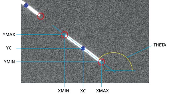
vi. THETA_IMAGE: Position angle (CCW/x, in degrees).
vii. XMIN_IMAGE: Minimum x-coordinate among detected pixels (in pixels).
viii. YMIN_IMAGE: Minimum y-coordinate among detected pixels (in pixels).
ix. XMAX_IMAGE: Maximum x-coordinate among detected pixels (in pixels).
x. YMAX_IMAGE: Maximum y-coordinate among detected pixels (in pixels).
and a new parameter, “line length”, is calculated as follows:
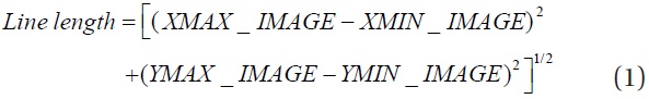
Fig. 5 shows an example of the application of “shape parameters” to a detected streak.
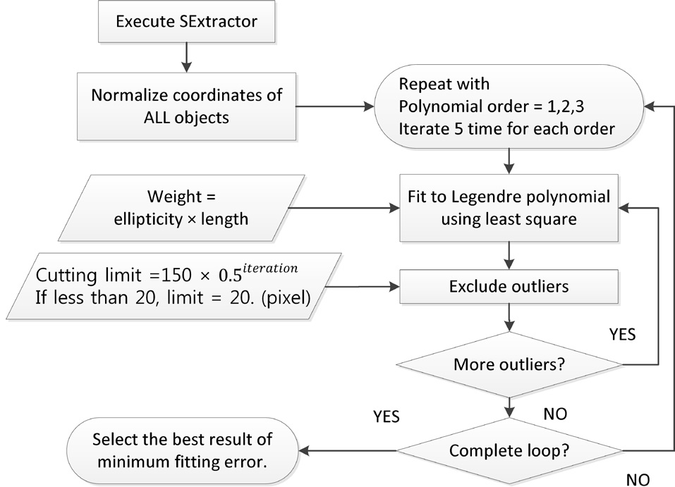
When a moving object is observed via the OWL detector system, it makes a group of multiple aligned streaks. These
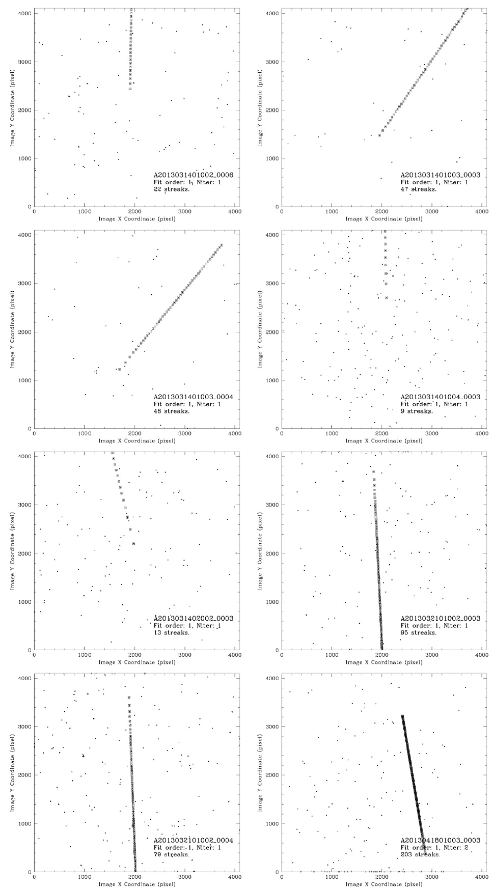
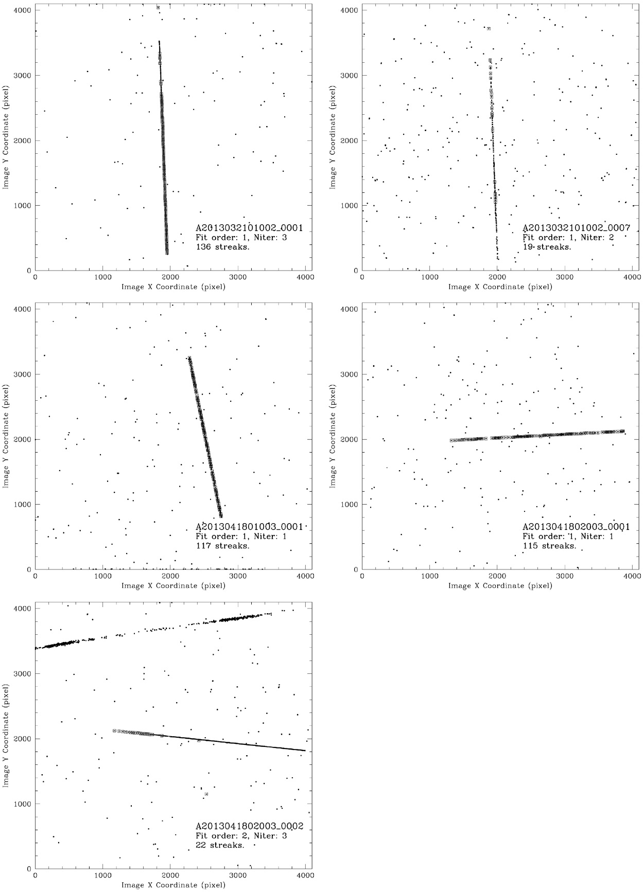
may be along a straight line, or a moderately bended curve. So, fitting the streaks with a curve can be a straightforward way to define the trace of a moving object on an OWL image. In Fig. 6, the flow of streak line fitting is outlined and Figs. 7 and 8 show examples of plotted streaks.
4.2 WCS solution calculation for coordinate transformation
After the positions of streaks are defined, the positions in image pixel X & Y values should be transformed into celestial coordinate values. The coefficients for this transformation are called world coordinate system (WCS) solution (Calabretta & Greisen 2002, Greisen & Calabretta 2002). To calculate these values, the pixel coordinate values of bright stars on the image frame must be compared with the celestial coordinate values in some published star catalogs like Guide Star Catalog (Lasker et al. 1990, Russel et al. 1990, Jenkner et al. 1990). Once the WCS solution is obtained, the positions of streaks can be easily defined in the form of right ascension & declination pairs.
WCSTools package (Mink 1997) is widely used to perform these tasks. It uses an amoeba algorithm, which is one kind of multi-dimensional downhill simplex method (Press et al. 1992), to find the most likely fit values of the coefficients. But as described in Section 3, OWL observation images don’t have sufficient numbers of bright stars to be used for this kind of trial-and-error of many possible cases because of the short exposure time of about less than 10 seconds. In addition, an amoeba algorithm needs initial values for all unknowns, and is very sensitive to them. So, we adopted IRAF (Valdes 1984) CCXYMATCH task which uses triangle pattern matching algorithm (Groth 1986) for matching image objects and catalog sources, and CCMAP task for calculating WCS solution from matched pairs found in CCXYMATCH.
Triangle pattern matching algorithm needs no initial values, and theoretically, only 3 suitably detected (bright, not saturated, not elongated) stars is sufficient to get to the goal.
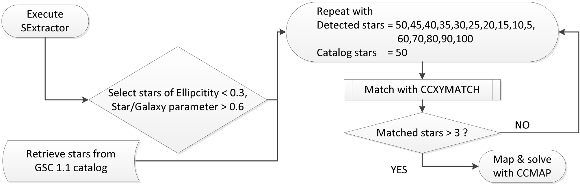
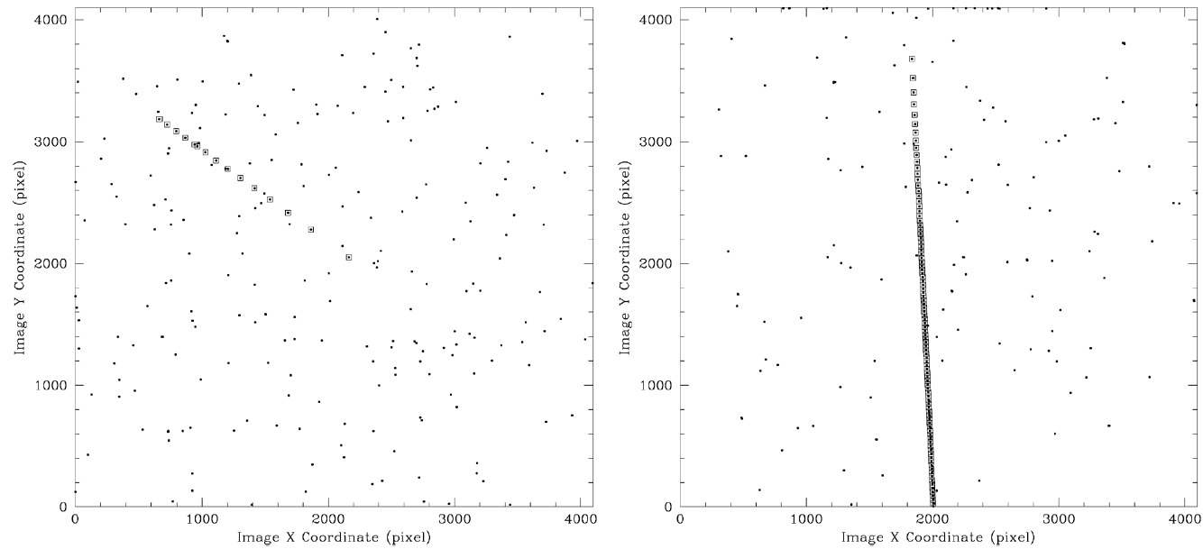
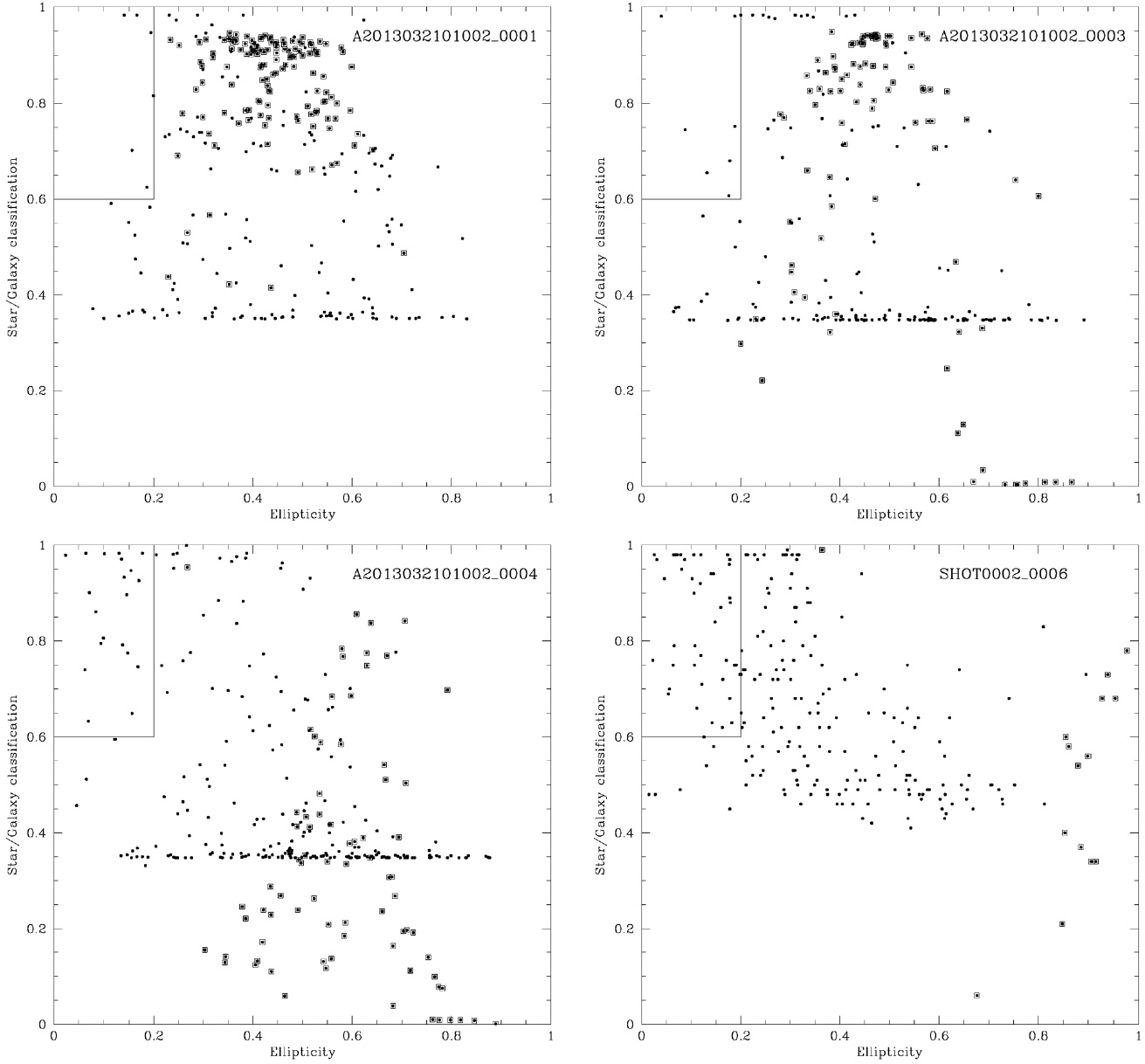
To calculate WCS solution coefficients using a triangle pattern matching algorithm, it is important to select ”good” background stars from SExtractor output. But this output also includes the streaks of moving objects. The basic idea of excluding streaks for WCS calculation input is shown in Fig. 9. In these figures, the boxed points are aligned streaks using the method described in Section 4.1. So, the remaining points (plain points) are background stars. From these, bright, not elongated (ellipticity < 0.2) and star-like (star/galaxy classification parameter > 0.6) objects can be used.
Fig. 10 depicts the flow of the WCS solution calculation procedure. Fig. 11 shows streak - eliminated background stars selected from an OWL image. Image pixel coordinate values of streaks should be transformed to topocentric equatorial (RA & Dec) values. This is done using the WCS solution coefficients and XY2SKY subprogram in WCSTools.
4.3 Combining positional data with time log data
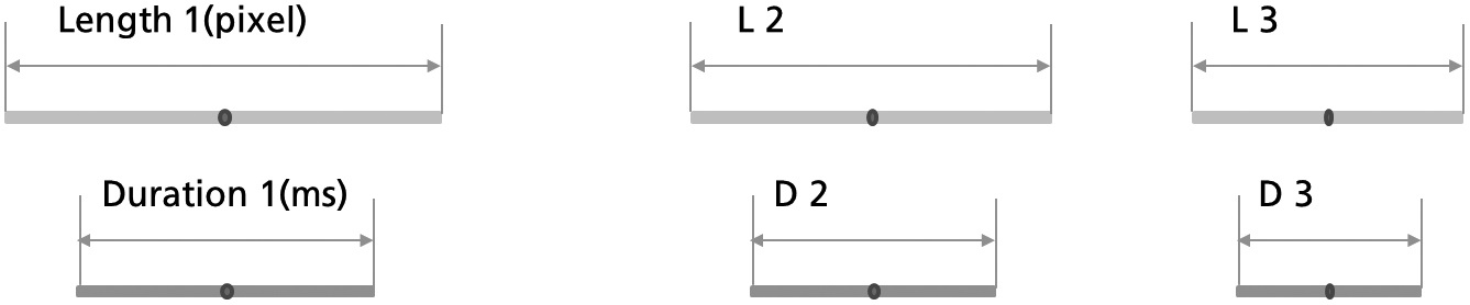
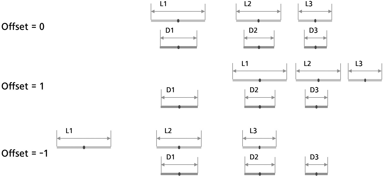
With the aligned streaks of a moving object and a set of time tagging log records, it is now possible to combine them and make a table of time - position for orbit analysis. It is clear that the length of a streak is proportional to the exposure time segment between obscurations by rotating chopper blades. Because the chopper starts to rotate, accelerates and finally reaches a stable speed, the streaks are relatively long, become shorter, and settle at a constant value. Therefore, the sequence of streak line lengths and the sequence of chopper open time segments can be matched using their relative ratios of line length versus chopper open time duration. This means that matching or combining two sequences will enable us to find the optimal offset between two sequences. The reference is the RMS standard deviation of (line length / time duration), L/D, normalized by the mean value of L/D. The concept of line length to the time duration ratio is shown in Fig. 12.
In other words,

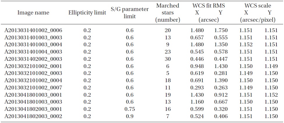
[Table 5.] Result of WCS solution calculation.

Result of WCS solution calculation.
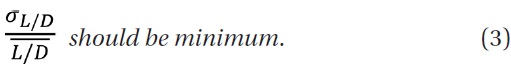

should be at its minimum for the best-matching sequence offset between line lengths and time durations. Fig. 13 shows how to match the offset of sequences of line lengths & time durations.
In this section, the reduction results of 13 images from Table 2 in Section 3.3 are presented.
As can be seen from Table 5, most of the cases can be solved with ellipticity of less than 0.2 and /G parameter greater than 0.6. Two exceptions are A2013041802003 0001 with S/G parameter greater than 0.75 and A2013041802003 0002 with S/G parameter greater than 0.9. In these two cases, the target was moving so slow and was so bright that the streaks are detected nearly as star-like objects. This meant that more strictly filtered background star lists for triangle pattern matching were required.
[Table 6.] Result of streak detection and line fitting.
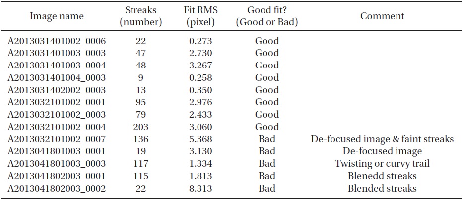
Result of streak detection and line fitting.
5.2 Streak detection and alignment
Table 6 shows the result of streak detection & line fitting, and Figs. 14 and 15 show the detected streaks for each images. Discussions of the “Bad” cases follow:
i. A2013032101002_0001: There are lost streaks from SExtractor detections. Because the background & noise level grows as the Y-coordinate increases due to the illuminations and the focus is not so good, some of the streaks of relatively big photometric errors (“MAGERR_AUTO” presented in Section 4.1) are excluded.
ii. A2013032101002_0007: There are lost streaks of big photometric errors due to bad focus.
iii. A2013041801003_0001: Some streaks are lost because they are not perfectly aligned along an ideal straight line. These look like the movement of a snake; that is, a twisting or curvy line. Possibly the target object (ARIANE 1 RB satellite debris) was rotating and so the sunlight reflection angle varied.
iv. A2013041802003_0001 & A2013041802003_0002: Blended streaks due to a bright & slowly moving target (RESURS DK 1 satellite) and an excessively fast chopper rotating speed (50Hz).
5.3 Streak position ? time data combination
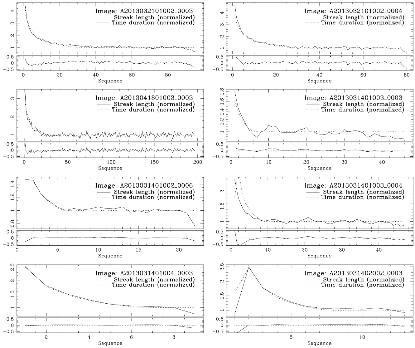
For “Good” cases in Table 6 and Fig. 14, we performed the streak position - time data combination procedure. In Fig. 16, normalized streak lengths vs. time durations with residuals are plotted. As expected in Section 4.3, the line lengths - time duration proportionality can be seen.
5.4 Coordinate transformation and final report
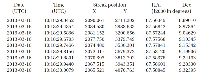
As described in Section 4, the image pixel coordinates are converted to topocentric right ascension and declination. The time log data is rearranged so that they indicate the midpoint of chopper open interval and add the chopper start time to make the final UTC time points. Table 7 is a sample result containing transformed coordinates and time data of streaks in the image A2013031401004 0003.
5.5 Influences of observation on OWL image data reduction
From the results seen so far, the quality or success rate of OWL image reduction has several dependencies on observational conditions.
i. Focus. As can be seen from Table 6, de-focusing increases the photometric errors in the brightness and the positional errors of sources detected using SExtractor. These poorly-detected sources might be forced to be included in the procedure of streak detection and alignment, but this will contaminate the result because many other normal (not streak) objects in a de-focused image can have larger errors than those in a well-focused image.
ii. Appropriate timing of exposure & chopper start. If the chopper starts too late, many of the position & time log data pairs can be lost.
iii. Sufficient brightness. As in the case of image A2013032101002_0001 in Table 6, if the streaks are too faint, they can be lost either at the stage of SExtractor photometry or line fitting. Increasing the aperture of the optics or rotating the chopper slowly can make the streaks brighter.
[Table 7.] Example final result of image A2013031401004 0003.

Example final result of image A2013031401004 0003.
OWL is an optical observation system for monitoring moving objects in the sky with a fast slewing & pointing mechanism, and a uniquely designed detector unit for maximizing the performance of acquiring positional and time data in relatively sort exposure time. During the period between March and April of 2013, we performed test observations on several clear nights, and took 13 good images and clean time log data for developing and testing the software algorithm of data reduction. Of these, 8 images could be analyzed in full depth, giving a total of 508 time - position data pairs. The remaining 5 images of the 13 were found to have minor problems, and this provided useful information for preparing future observations. By using this algorithm and good quality image & time data, the basic input data can be produced for efficiently determining the orbit of moving objects, such as artificial satellites and space debris.