Photometric light variation is one of the types of information that is useful for detecting the relative position and characteristics of space objects. Pavlenko (2012) developed an algorithm related to the estimation of a satellite’s rotational parameters. Using this method, space debris and satellites are also investigated and identified in near-Earth space. The photometric response type was studied statistically from a large database to categorize the satellites (Hejduk 2010). Fig.1 in Hejduk (2010) shows that if a body is a purely specular sphere, brightness does not change with phase angle for a diffuse-specular sphere. Payne et al. (2007) also measures color photometry to determine identity and characteristics, and the color photometry is separated by type of payload and satellite. In addition, different satellites have different colors and brightnesses. Multiband optical photometric observation supplies information about the spacecraft’s position, attitude and material properties (Jah & Madler 2007, Hall 2010). This photometric observation is also one of the important methods to determine empirical interpretation and shape for all asteroids, including near Earth asteroids (Kaasalainen & Torppa 2001).
In this paper, we compared the results of our simulation of photometric light variation with an optical observation to investigate the correlation between light variability and satellite shape. For this research, we selected the Communication, Ocean, Meteorological Satellite-1 (COMS-1) satellite which has a well-known position and morphology. We describe our phase angle calculation method for brightness calculation in Section 2. The observation data analysis is in Section 3 and an estimated light variation and brightness are presented in Section 4. In Section 5, we discuss the results of comparing the light variation of the COMS-1 Geostationary Orbit Satellite (GEO) satellite with our observation data.
Satellite brightness depends on the reflection angle of the Sun’s light, as well as on the relative angle of observer-satellite-SUN. A phase angle is defined as the angle between the light incident onto an observed object and the light reflected from the object. In this paper, the phase angel means the angle of Observer-satellite-SUN. To estimate the variation in brightness over time, we calculated phase angle through the following method. The phase angle (
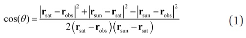
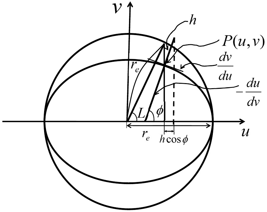
where, rsun is the position of the sun, rsat, is the position of the satellite, and robs is the position vector of the observatory. We employed a series expansion formula to calculate the position of the Sun (Montenbruck & Gill 2000). To calculate the observational position, we used an observatory position determination method including the ellipsoidal model of Earth (Fig. 1) and using Eq. (2) (Kim 2005).
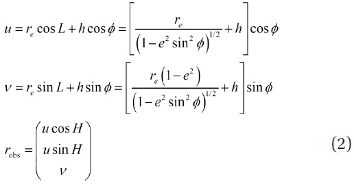
re: Earth equatorial radius
L: Geocentric latitude
φ: Geodetic latitude
e: Eccentricity of earth
h: Sea level height
H: Local siderial time
The initial value of orbital elements is determined by employing Two-Line Element which was released by Joint Space Operation Center, located at Vandenberg Air Force Base in California.
We calculated the time varying three elements (Ω, ω, M) including
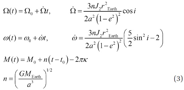
a, e, i, Ω, ω, M: Keplerian Orbital Elements
MEarth: Earth’s mass
G: Gravity constant
J2: Gravity Harmonics
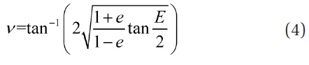
To display the real position of the satellite in the satellite-based coordinate system, we derived the true anomaly
E-esinE=M(t), E:eccentric anomaly
After that, we converted the satellite’s position in the satellite coordinate system into GCRS, as shown in Eq. (5) as follows (Wiesel 1997, Vallado 2007).
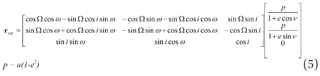
Finally, we were able to obtain the phase angle θ from equation 1 with the three parameters (robs, rsat, rsun) derived through the above equations. Therefore, the minimum
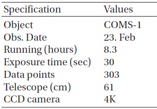
[Table 1.] COMS 1 observation log.

COMS 1 observation log.
value of θ is found by repeating calculations in every time span within the given period.
We examine the phase angle variance from Feb. 23rd, 2011 21:00 to Feb. 24th, 2011 09:00 (KST) to compare with photometric observation. In this calculation, the minimum phase angle of COMS-1 shows 15.72˚ at 2455616.1528 JD (Feb. 24th, 2011 00:40:02 KST ).
To verify our brightness calculations, observation was carried out with a 61 cm telescope at Sobaeksan Optical Astronomy Observatory. For this observation, the telescope was operated in non-sidereal tracking mode. But we took a few frames in tracking mode to obtain instrumental magnitude at around maximum brightness time. We obtained a time series of CCD images through an R bandpass filter with a 4K CCD camera system. This photometric observation is summarized in Table 1.
Instrumental magnitudes were obtained using the simple aperture photometry routine in the IRAF APPHOT package. The aperture radius was chosen as 6˝. We then calculated differential brightness change of the COMS satellite. In this observation, we did not compare the brightness difference between the comparison star and this target satellite for all of the observation data points because an absolute magnitude was not required in this research. But the maximum instrumental magnitude was derived from nearby comparison star magnitude. Air mass was also not considered in our data processing because a geostationary satellite is located at a fixed point location in a horizontal coordinate, which means it is not a serious factor in brightness change. But the sky brightness is subtracted in aperture photometry.
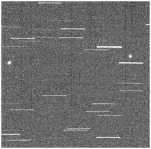
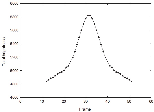
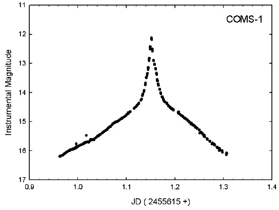
Fig. 2 shows the COMS-1 light curve made from observation data on Feb. 23rd, 2011 at Sobaeksan astronomical observatory. Fig. 3 is one of our COMS-1 observation image frames.
The observed time of maximum brightness is derived from polynomial quadratic curve fitting with symmetrical minimum brightness. The calculated maximum brightness peak time is 2455616.1518 (JD) in our observation. The time
difference shows 0.001 days between observation data and a numerical calculation in previous Section 2. We think that the time difference is caused by other factors such as satellite attitude, solar panel position and coordinate differences.
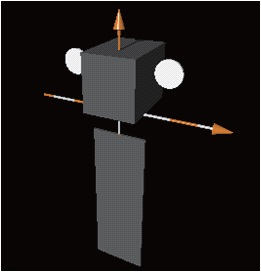
For the estimation of COMS-1 brightness variation, we used a rendering method with Persistence of Vision Raytracer software. Fig. 4 shows a rendering model that
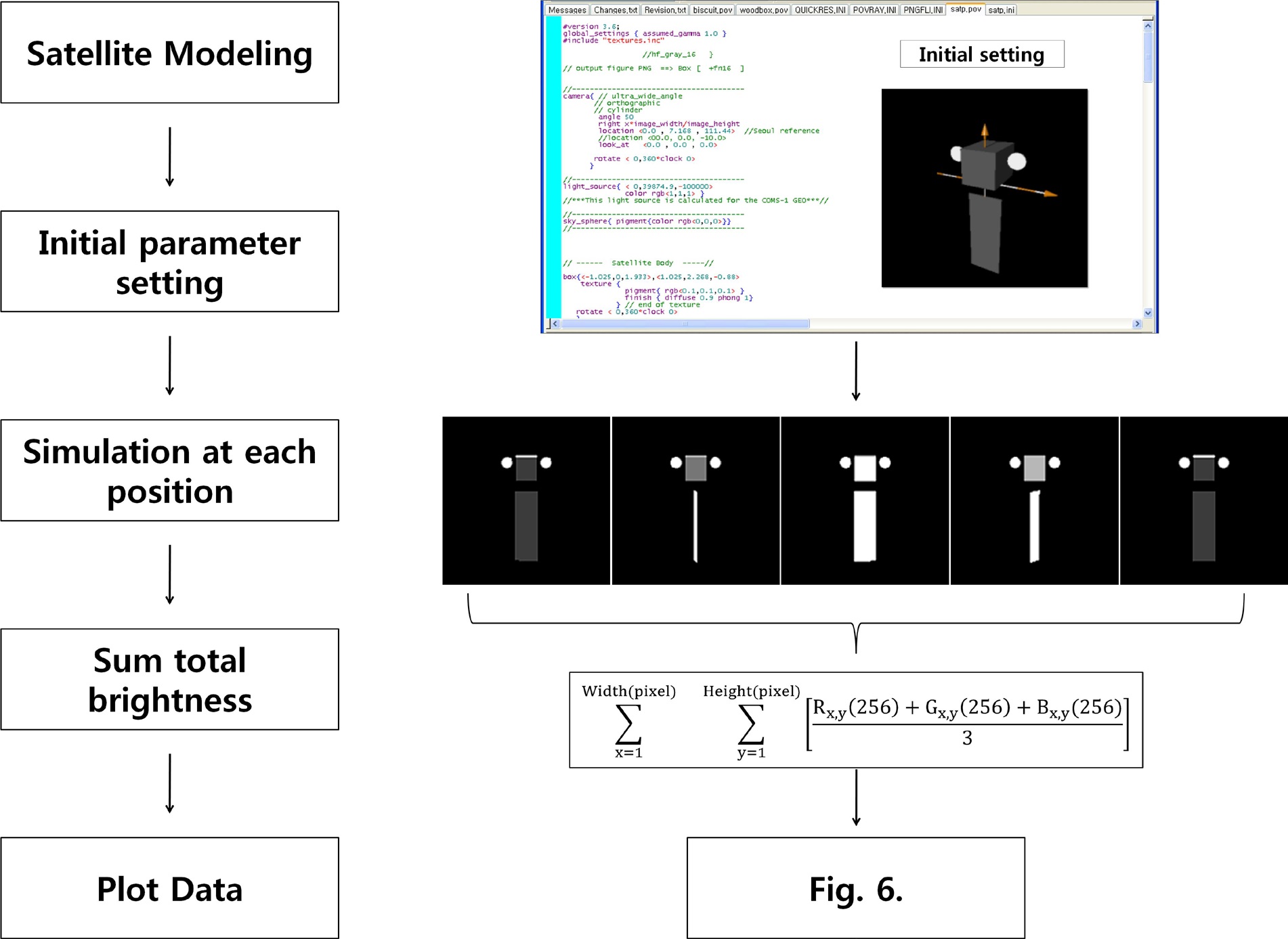
is designed with a simple box shape based on the COMS-1’s dimension. The simple box shape represents the characteristic structure of solar panel, bus, antenna (The arrows in the figure have no meaning). The surface texture parameter of the satellite consists of {r(0.1), g(0.1), b(0.1)} and 0.9 diffusion with the Phong 1 model. The Phong 1 model is applied when the reflection is stronger in one viewing direction, such as in a bright spot. The camera position and SUN angle are set to spatial ratio at spring time in South Korea. This simulation is able to generate a bitmap file at each position. Therefore, we can estimate the total brightness from each bitmap figure. The brightness is calculated based on the sum of all pixels from the bitmap file. In this study, we use a PNG gray scale bitmap file because we only need the total brightness. Fig. 5 shows a process of rendering model analysis. The first step is to draw the simple structure of the satellite. The second step is to define the surface texture parameter. The third step is to rendering each rotating position. In this model, we assumed that solar panel rotated by following the Sun’s direction. The
fourth step is to find the summation of each pixel value of the bitmap file. The final step is to obtain the light curve.
The variation in brightness of the rendering model
is shown in Fig. 6. The x-axis is divided into one Earth rotation by 60 frames. The brightness value can also change according to camera distance value in the software but we just use the normal distance value to know the shape of a brightness change in this model. From this result, the COMS-1 satellite shows that the brightness shape has one peak and rapidly decreasing wings.
We calculated the brightness of the satellite using Hedjuk’s equations induced from Pogson’s equation (Hejduk 2007, 2011). The equations include phase function (
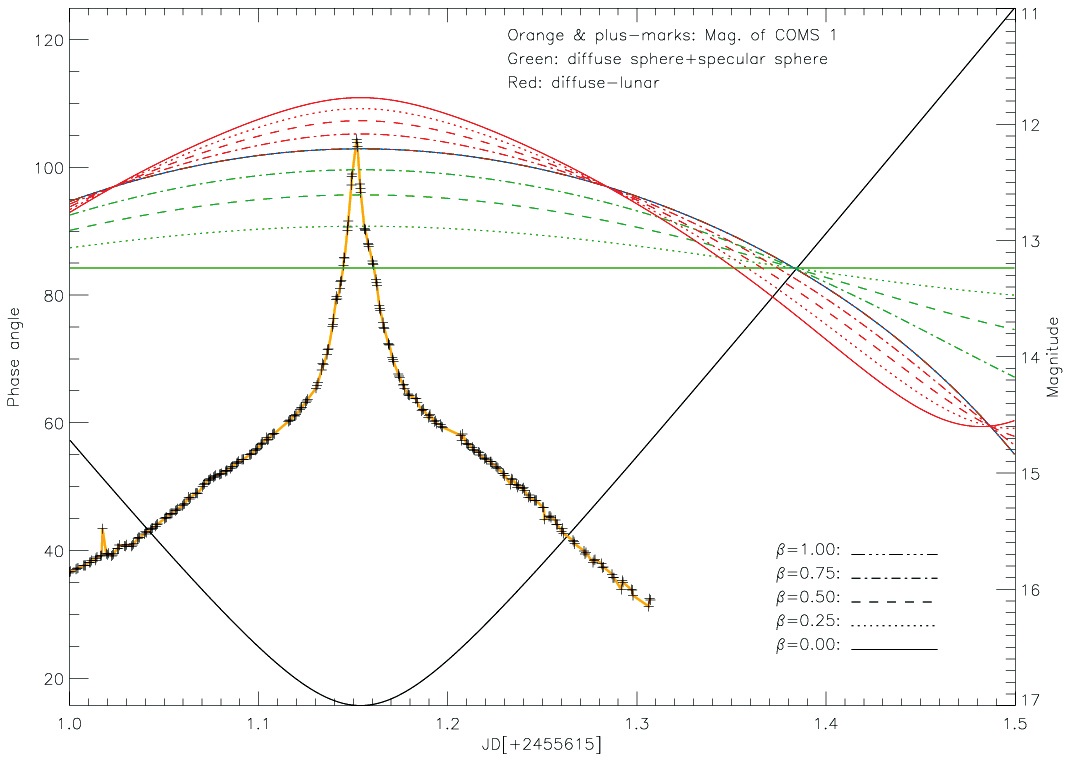
The albedo of the satellite varies depending on the construction material used and its scattering properties. Certain satellites can present a value from 0.0 to 0.5 (Hejduk 2011), and most satellites have a value of 0.1. So we substitute 0.1 for the albedo, and the albedo of the satellite does not always correspond to the satellite’s size (Henize et al. 1993). The satellite’s size in this paper means the size of the solar panel, not the total size of the satellite. Eq. (6) is the basic function for the brightness calculation of a satellite using the apparent magnitude of Sun for comparison (Wiesel 1997), and the result is shown in blue in Fig. 7.

A: cross-sectional area
ρ: satellite’s bond albedo
φ: phase angle (in radian)
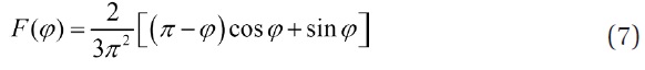
F(φ): phase function
R: the distance from observer
The phase function (Eq. (7)) is based on Mulrooney’s study of phase function for fragmentation debris (Mulrooney 1993). Most objects are neither a pure diffuse sphere, nor a pure specular sphere, so the two phase functions have to be combined. We calculated the brightness using the combined phase functions. The method is called the “diffuse-specular model”, and β is the mixing ratio of the two phase functions. The green lines in Fig. 7 show the computational results. The solid line (β = 0) in green means the pure specular sphere, and the dot-dot-dot-dash line (β = 1) in green means the pure diffuse sphere in Fig. 7. When phase angle is less than 90°, pure diffuse sphere is brighter than pure specular sphere, and when phase angle is more than 90°, the opposite trend appears. The model of diffuse-specular sphere indicates the degree of reflection with phase angle. In this model brightness variation does not appear the case of the specular sphere (β = 1) (Hejduk 2010).
The Moon also affects the satellite’s brightness, so the calculation has to take the Moon’s effect into account. The satellite’s brightness of diffuse sphere is decreased by the full Moon, because the full Moon is brighter than a diffuse sphere. The brightness equation is applied to the phase function considering the Moon’s effect, and the red lines in Fig. 7 show the results with β. Solid line (β = 0) in red color means pure lunar effect, and dot-dot-dot-dash line (β = 1) in green color means diffuse-lunar sphere in Fig. 7. When phase angle is 0° ~ 50°, diffuse-lunar sphere is brighter than pure diffuse sphere, and when phase angle is 50° ~ 120°, the reverse occurs. The diffuse-lunar model refers to the effect of lunar reflection. In this model brightness variation is larger over time, in the case of diffuse-lunar (β = 1).
The solar phase angle of the COMS-1 was computed by Jin et al. (2011), and the calculation is explained in Section 2. The distance from the satellite to the observer (Earth) is 36,000 km, the altitude of COMS 1.
Maximum brightness of the modeling result matches with observational data, but the wings of graphs are different for each line shape. We think that because in brightness calculation we considered the solar phase angle, albedo, size of satellite, and distance while ignoring residual conditions, the two graphs, observational data and result from calculation, are different.
We investigated the variation in brightness of the COMS-1 GEO satellite to determine the characteristics of space objects through optical observation. For the investigation of the shape of the brightness variation and the maximum brightness, we compared the observation result with our estimated calculation and a rendering simulation. In the case of COMS-1, the light curve shows a single peak in our model and observation because the surface orientation of the satellite body and the two antennas are on the line of sight between the observer and satellite. The estimated maximum brightness is close to 12.1 magnitude compared with our observation, and the time difference is 0.001 days. This simulation and brightness calculation shows reasonable results. This research will be an aid to future study of the features of satellites and space objects using their brightness.