검색 전체 메뉴
PDF
맨 위로
OA 학술지
Development of indirect EFBEM for radiating noise analysis including underwater problems
  • 비영리 CC BY-NC
  • 비영리 CC BY-NC
ABSTRACT
Development of indirect EFBEM for radiating noise analysis including underwater problems
KEYWORD
Energy flow boundary element method (EFBEM) , Radiating noise , Free surface effect , Directivity factor.
  • INTRODUCTION

    When ships or underwater objects move through water, whose impedance is much higher than that of air, small vibrating motions of the inner ship body can cause remarkable noises in wide frequency ranges. No single analysis method of the noise phenomenon can be effectively applied to all ranges of noise problems. At low frequency ranges, the analysis of vibration problems is analyzed by the conventional methods such as the Finite Element Method (FEM) and Boundary Element Method (BEM). But, at high frequency ranges, those methods require more computation time and costs, and thus alternative methods are needed.

    Among many alternative methods, EFA has received much attention. This method was introduced by Belov et al. (1997) in 1997. Nefske and Sung (1989) implemented Energy Flow Finite Element Method (EFFEM) to solve the transverse vibration of a beam. Wholever and Bernhard (1992) derived the energy governing equation for diverse vibrating waves of a beam. Bouthier and Bernhard (1992) derived the energy governing equation of a flexural wave, considering only the far-field component of the transverse vibration of a membrane and thin plate. They expanded the research of EFA to vibration problems of twodimensional structures. Cho (1993) researched the energy boundary condition in the connection point between elements of a beam by applying the wave transmission approach to a complex structure. Park (1999) and Park et al. (2001) derived the energy governing equation for an in-plane wave of a thin plate and studied the spatial distribution and transmission path of vibration energy for a plate structure, which is connected at a non-determined angle. Seo et al. (2003) expanded the application of EFA to beam-plate coupled structures. Lee et al. (2008) applied EFBEM to the vibration analysis of beam and plate problems. Also Wang et al. (2004) applied energy boundary element formulation to the sound radiation problems.

    In this paper, the energy governing equation having spherical wave property is developed in open field. And the directivity effect which is represented in high frequency range problems but can’t express in EFA is studied. And the fundamental solution and energy governing equation for underwater problems are developed. The developed equation and directivity effect are applied to the simple case and the results are compared with commercial noise analysis program, SYSNOISE and reliable results are obtained.

    ENERGY GOVERNING EQUATION FOR RADIATING NOISE ANALYSIS

      >  Energy balance equation

    In a linearly elastic medium, the energy balance equation is derived from the following Eq. (1). The amount of incoming and out coming power through the surface of an object and the rate of change of the total energy in the object are same. From this fact, energy balance equation is represented as follows:
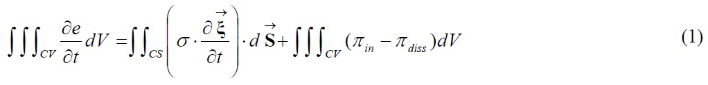
    image

    where, e is the total energy density in the volume of an object, CV.

    image

    is the displacement vector at the boundary of an object, CS.

    image

    is a small area vector perpendicular to the surface of the boundary.
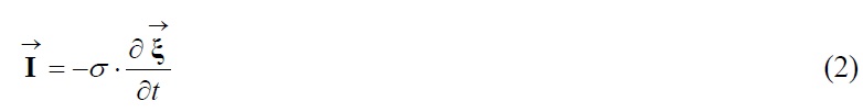
 σ represents the stress on the surface of the boundary. πin and πdiss are expressed as input power and loss power acting on a unit volume at a unit time, respectively. Intensity, defined as the power per unit area flowing out of an object, can be obtained from the stress acting on the surface of the boundary and the velocity of the surface of the boundary as follows:

    image

    where,

    image

    is the intensity, the power per unit area. In Eq. (1), the first integral on the right hand side is rewritten with the application of Gauss’s theorem as follows:

    image

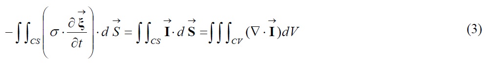
    Therefore, the energy balance equation in the volume of an object is obtained by

    image

    From Eq. (4), the energy balance equation for a small volume is expressed by

    image

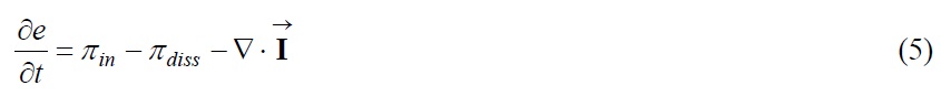
    Eq. (5) is the energy balance equation for all elastic mediums, steady state and transient state. For a steady state elastic medium, the rate of energy density with respect to the time is zero; the left term in Eq. (5) is zero. Therefore, the steady-state energy balance equation is represented as follows:

    image

    From Eq. (6), the input power due to the exterior exciting force is expressed as the sum of the power lost in the object and the power flowing out the adjacent medium.

      >  Energy loss equation

    The loss of vibration energy can be represented by a damping structure model. Cremer et al. (2004) showed that energy density loss, ediss, due to the damping structure per one period at any point in an elastic medium vibrating at frequency ω is proportional to reversible vibration energy density, eR. Therefore, Eq. (7) is obtained by

    image

    If the inner damping coefficient η is very small, the reversible energy density, eR, can be substituted for the time average value of the total energy density, <e> , which is the sum of the kinetic energy density and the potential energy density. Therefore, Eq. (8) is given by

    image

    where, < > means the time average. The time average of power loss during one period, <πdiss> can be obtained by dividing the energy loss during one period, ediss by period, T being 2π/ω. And it can be obtained approximately by using the time average of the total energy density, <e>, as follows:

    image

    Eq. (9) is the energy loss equation, which is derived from the application of structural damping to any point on an elastic medium vibrating at frequency ω. We assumed that the kinetic energy is the same as the potential energy.

    ENERGY GOVERNING IN UNDERWATER RADIATING NOISE ANALYSIS

      >  Energy transmission equation in underwater radiating noise analysis

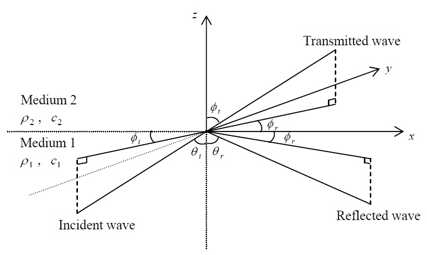
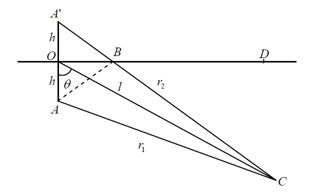
    For analyzing the radiating noise problems underwater, we must consider the effect of free surface. According to Fig. 1 and reflection coefficient of surface, spherical wave in underwater is represented as follows:

    image

    where, r1 is the direct distance between a source point and field point. r2 is the distance arrived from the source point to the field point which is reflected at the free surface of the water.

    image

    is the wave number considering the damping effect. η is damping loss factor and k is the wave number. From the Euler’s equation, the velocity of the wave can be obtained.

    Therefore, energy density and intensity can be expressed as follows for a far-field with low damping:

    image
    image

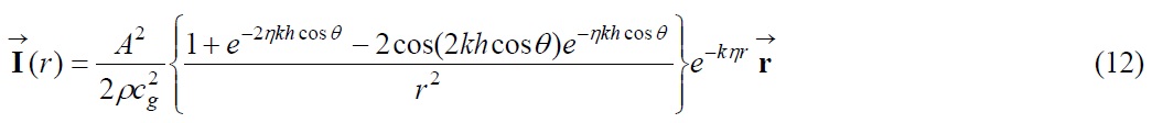
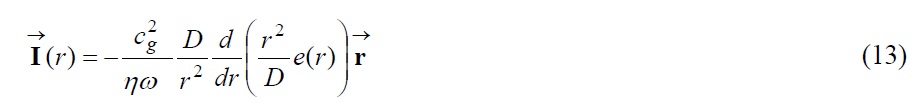
    From Eqs. (11) and (12), the following energy transmission equation can be obtained as follows:

    image

    where, D = 1 + e-2ηkhcosθ ?2cos(2khcosθ)e-ηkhcosθ.

      >  Energy governing equation in underwater radiating noise analysis

    From the energy balance equation, Eq. (6), the energy loss equation, Eq. (9), and the energy transmission equation, Eq. (13), the energy governing equation can be obtained as follows:

    image

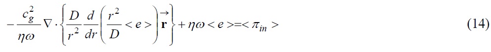
    Eq. (14) is the energy governing equation representing the property of a spherical wave and including the effect of the water surface.

    DERIVATION OF THE FUNDAMENTAL SOLUTION IN UNDERWATER RADIATING NOISE ANALYSIS

    The fundamental solution G is the exact solution for input power, as well as the fundamental solution representing the relation between the virtual source and energy density. Therefore, the shape of the fundamental solution G corresponds to that of the energy density of Eq. (12). According to this equation, the fundamental solution G is expressed as follows:

    image

    Fundamental solution H representing the relation between the virtual source and intensity is obtained from Eq. (14) as follows:

    image

    When intensity boundary condition is applied to Eq. (16), the value of C1 is obtained as follows:

    image

    In the left term of Eq. (17), the integral of

    image

    is equal to one, because of the property of the Dirac delta function, δ(r). According to this property and Eq. (16), Eq. (17) is expressed as follows:

    image

    In the right term of Eq. (18), D remains. The e-2ηkhcosθ ?2cos(2khcosθ)e-ηkhcosθ term of D represents the effect of the reflected wave. If radius approaches zero, this effect diminishes; that is, D=1. Therefore, C1 can be obtained from Eq. (18) as follows:

    image

    From Eq. (19), we know that the non-determined constant C1 is

    image

    Therefore, the fundamental solution representing the relation between the virtual source and energy density or intensity is as follows:

    image

    Eq. (20) is the fundamental solutions having the property of a spherical wave and incorporating the effect of the water surface.

    DIRECTIVITY FACTOR

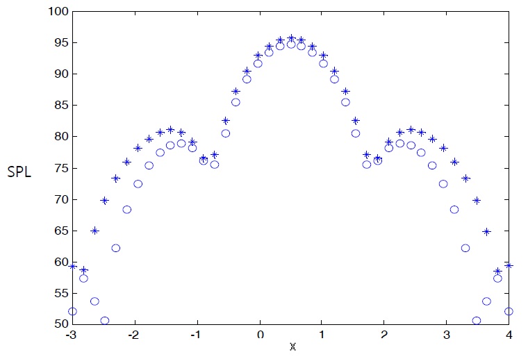
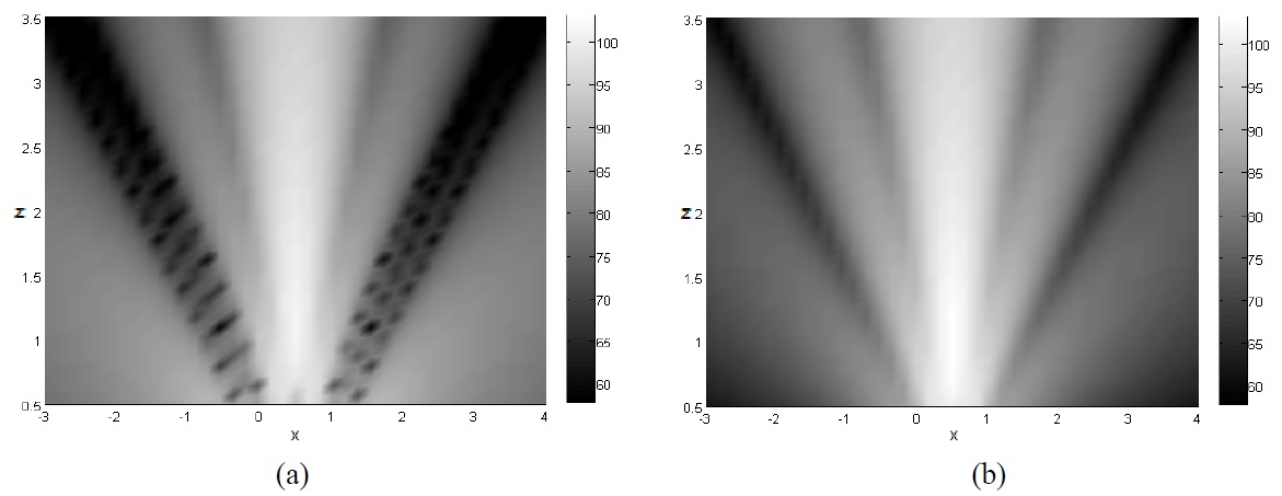
    BEM which is one of traditional noise analysis methods shows the noise’s directivity pattern at high frequency ranges. This is caused by the difference of wave’s phase. But EFA doesn’t show the noise’s directivity pattern, because EFA doesn’t have the phase information. So representing the noise’s directivity, the directivity factor is developed.

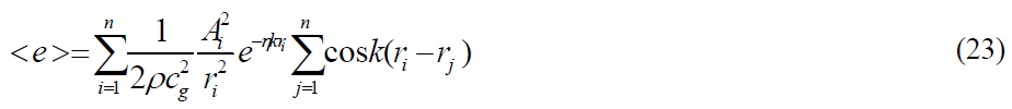
    When n sources are existed, the energy is as follows:
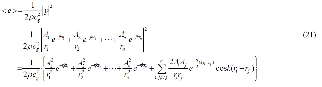
    image

    Here

    image

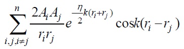
    is newly added. This equation can be divided to two terms as follows:

    image

    From Eqs. (21) and (22), the following equation can be obtained as follows:

    image

    where

    image

    is directivity factor.

    ESTABLISHMENT OF BOUNDARY INTEGRAL

      >  Establishment of boundary integral for indirect method

    In the indirect method of the boundary element, the real system of finite size is extended to the infinite field and the virtual source is assumed to exist on the boundary of the real system. And energy and intensity in the concerned field are obtained by using fundamental solution as the sum of the effects due to virtual sources. Based on this concept, in three-dimensional problems, equations of energy density and intensity are obtained in the concerned field as follows:

    image
    image

    where, V is assumed as the concerned field in three dimensions and S is assumed as the boundary surface encompassing the concerned field. The fundamental solution, G and H has the same shape as that of Eq. (20).

    image

    indicates a field point of the concerned field.

    image

    means the position of the virtual source on the boundary.

    image

    is the location of input power.

    image

    means the virtual source on the boundary surface. The virtual source on the boundary surface,

    image

    can be obtained by using Eqs. (24) and (25) according to the property of the boundary condition. If

    image

    approaches the boundary surface, the boundary integral of the right term in Eqs. (24) and (25) has a singular integral whose point is centered on the boundary surface. This point is the identity of

    image

    Therefore, the integral term of the Eq. (24) is divided into the following terms as follows:

    image

    where, if the boundary of the concerned field is a smooth curve surface, the boundary surface Sε is a hemisphere with the small radius ε, centering on the boundary point. And the boundary surface SSε indicates the part which is subtracted from the boundary surface Sε from total boundary surface S. The first right term of the Eq. (26) is as follows:

    image

    where, if the radius ε approaches zero, the area of the boundary surface Sε becomes 2πε2. So Eq. (28) is obtained by taking the limit of Eq. (27) as follows:

    image

    And if radius ε approaches zero, the boundary integral term with respect to the boundary surface SSε, is replaced with the boundary integral with respect to the total boundary surface, S. Eq. (27) is expressed about one point on the smooth boundary surface as follows:

    image

    APPLICATION

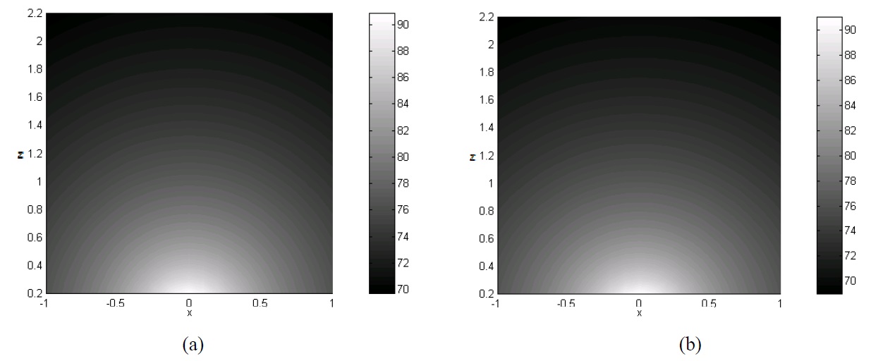
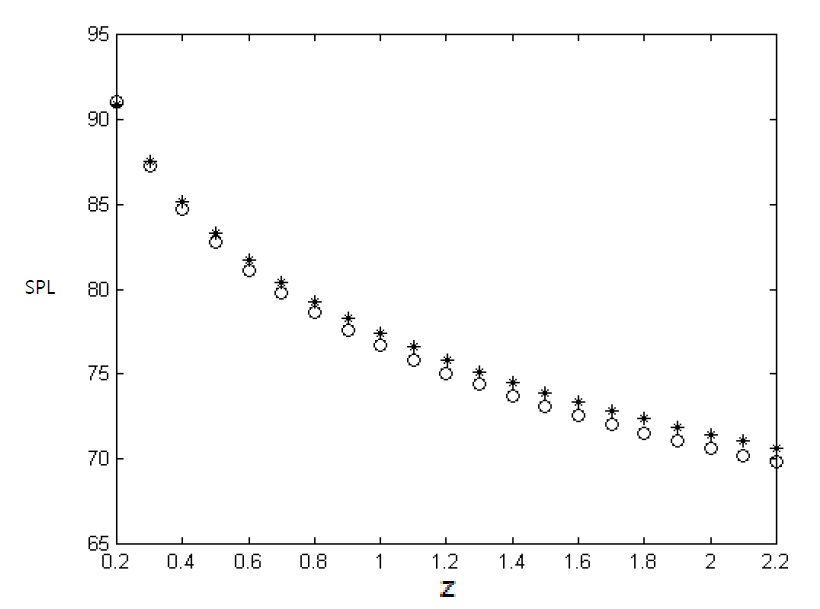
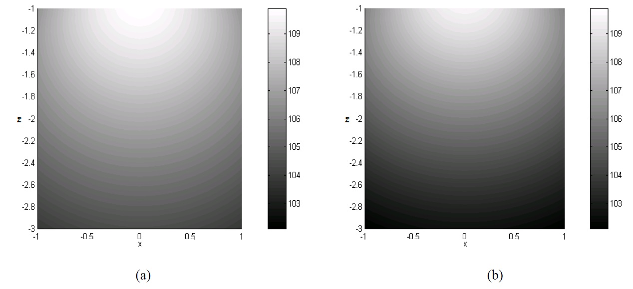
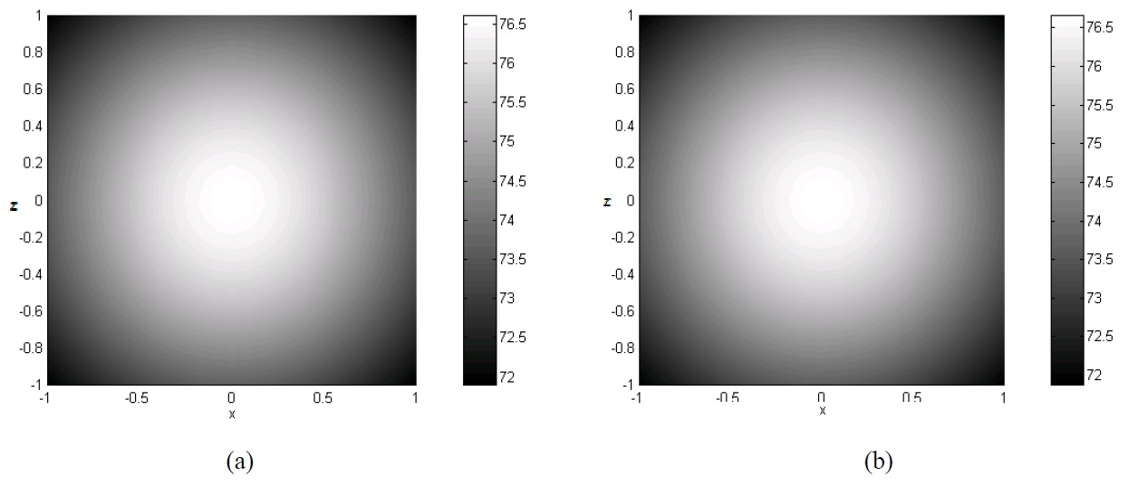
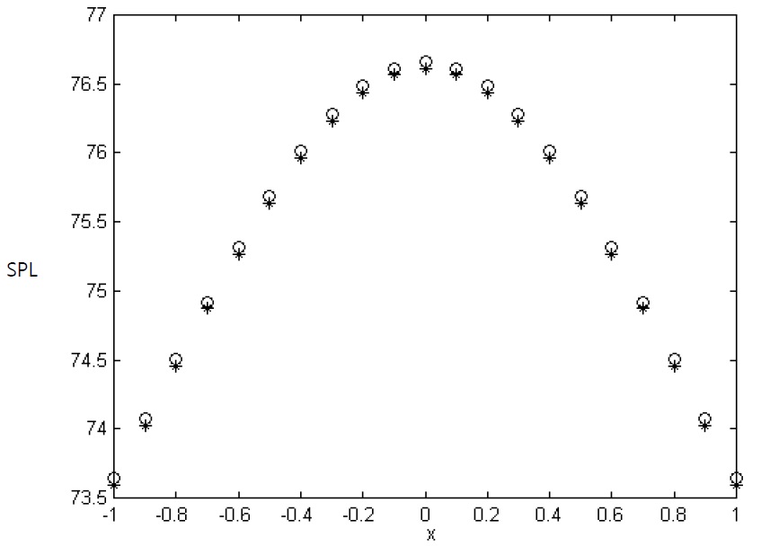
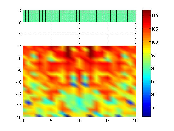
    EFA is developed by assumptions which are high damping value and medium-to-high frequencies. According to these assumptions, the nearfield evanescent waves can be neglected. So EFA’ s result is not good agreement with a classical solution at low damping values, because the effect of nearfield waves will be affected on the vibration phenomena in low damping system. Therefore EFBEM will be applied to the high damping systems. To verify the accuracy of the developed works, the boundary integral of indirect EFBEM was applied to the radiating noise problems of structures with the vibration of a simple plate model and a simple sphere model in open field and underwater. And the result of the indirect EFBEM was compared with that of SYSNOISE. Figs. 3 and 4 show energy density distribution, respectively, in the z-direction by SYSNOISE and indirect EFBEM when the plate which size is 1 m × 1 m, is located at x-y plane when f is 1 kHz, v is 0.1 m/s and η is 0. Field points which size 7 m × 3 m is located x-z plane. Though EFBEM can consider the damping loss factor in a medium, a damping loss factor of zero was used so that EFBEM could be compared with SYSNOISE. Fig. 5 shows a simple sphere structure which radius is 0.5 m, with a uniform vibration in open field. When f is 1 kHz, v is 0.1 m/s and η is 0, Figs. 6 and 7 show the energy density distributions, respectively, in the z-direction by SYSNOISE and indirect EFBEM when the sphere is located under the field points. Field points’ size is 2 m × 2 m. Figs. 8 and 9 show the energy density distribution in the x-z plane predicted by SYSNOISE and indirect EFBEM when the sphere is set at the center of the field points. From Figs. 3,4, and 6-9, we can see that the results of indirect EFBEM agree with those of SYSNOISE in open field. Fig. 10 shows the energy density distribution in the zdirection predicted by SYSNOISE and indirect EFBEM when the sphere is located near the water surface. Though the difference of the results between SYSNOISE and indirect EFBEM is about 1 dB, the patterns of the results are the same. Fig. 11 shows a simple barge type structure with a uniform vibration in open field. When f is 63 Hz, v is 0.1 m/s and η is 0, Fig. 12 shows the energy density distributions, respectively, in the z-direction by SYSNOISE and indirect EFBEM when the barge type structure is located above the field points. Though the difference of the results between SYSNOISE and indirect EFBEM is about 5 dB, the patterns of the results are the same. And Fig. 13 shows the energy density distribution when f is 1 kHz, v is 0.1 m/s and η is 0. Because the barge type structure is large, SYSNOISE can’t analyze noise analyses but EFBEM can analyze those over 1 kHz.

    CONCLUSION

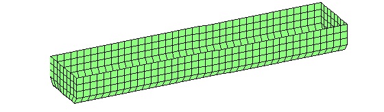
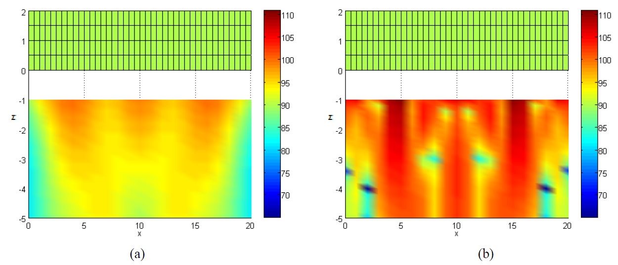
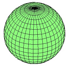
    This paper analyzed radiating noise problems in the medium-to-high frequency range. The energy governing equation and fundamental solutions having the spherical wave property were developed. And the directivity which was the property of high frequency analysis but couldn’t represent in existing EFA, was developed. Also, the fundamental solutions representing the effect of the water surface were developed for the underwater radiating noise problems. Last indirect EFBEM applying BEM to EFA was developed for this analysis. To verify the developed works, the results of the indirect EFBEM were compared with those of commercial code, SYSNOISE in open field. For plate, the directivity was represented similar shapes in SYSNOISE and developed indirect EFBEM. And the directivity was vanished for sphere model. Also the effect of the water surface was examined by the comparison of the results between indirect EFBEM and SYSNOISE for an underwater case. These comparisons showed satisfactory results and developed indirect EFBEM is applied to barge type structure at high frequency.

참고문헌
  • 1. Belov V.D., Rybak S.A., Tartakovskii B.D. 1977 Propagation of vibrational energy in absorbing structures. [Soviet Physics Acoustics] Vol.23 P.115-119 google
  • 2. Bouthier O.M., Bernhard R.J. 1992 Models of space-averaged energetics of plates. [American Institute of Aeronautics and Astronautics Journal] Vol.30 P.616-623 google cross ref
  • 3. Cho P.E. 1993 Energy flow analysis of coupled structures. google
  • 4. Cremer L., Heckl M., Petersson B.A.T. 2004 Structure-borne sound. google
  • 5. Lee H.-W., Hong S.-Y., Park D.-H., Kwon H.-W. 2008 Energy flow boundary element method for vibration analysis of one and two dimension structures. [Shock and Vibration] Vol.15 P.33-50 google
  • 6. Nefske D.J., Sung S.H. 1989 Power flow finite element analysis of dynamic systems : basic theory and application to beams. [Journal of Vibration, Acoustics, Stress and Reliability in] Vol.111 P.94-100 google cross ref
  • 7. Park D.H. 1999 Vibration power flow analysis of coupled plates and box-type structures. google
  • 8. Park D.-H., Hong S.-Y., Kil H.-G., Jeon J.-J. 2001 Power flow model and analysis of in-plane waves in finite coupled thin plates. [Journal of Sound and Vibration] Vol.244 P.651-668 google
  • 9. Seo S.-H., Hong S.-Y., Kil H.-G. 2003 Power flow analysis of reinforced beam-plate coupled structures. [Journal of Sound and Vibration] Vol.259 P.1109-1129 google
  • 10. Wang A., Vlahopoulos N., Wu K. 2004 Development of an energy boundary element formulation for computing high-frequency sound radiation from incoherent intensity boundary conditions. [Journal of Sound and Vibration] Vol.278 P.413-436 google
  • 11. Wohlever J.C., Bernard R.J. 1992 Mechanical energy flow models of rods and beams. [Journal of Sound and Vibration] Vol.153 P.1-19 google
OAK XML 통계
이미지 / 테이블
  • [ Fig. 1 ]  Wave propagation from medium 1 to medium 2.
    Wave propagation from medium 1 to medium 2.
  • [ Fig. 2 ]  The distance between field point and source point.
    The distance between field point and source point.
  • [ Fig. 3 ]  The energy density distribution in z-direction when the plate is vibrating: (a) SYSNOISE, (b) Indirect EFBEM.
    The energy density distribution in z-direction when the plate is vibrating: (a) SYSNOISE, (b) Indirect EFBEM.
  • [ Fig. 4 ]  The energy density distribution in z-direction when the plate is vibrating: *, SYSNOISE; o, Indirect EFBEM.
    The energy density distribution in z-direction when the plate is vibrating: *, SYSNOISE; o, Indirect EFBEM.
  • [ Fig. 5 ]  Uniformly vibrating 3-dimensional spherical structure.
    Uniformly vibrating 3-dimensional spherical structure.
  • [ Fig. 6 ]  The energy density distribution in z-direction when the sphere is vibrating: (a) SYSNOISE, (b) Indirect EFBEM.
    The energy density distribution in z-direction when the sphere is vibrating: (a) SYSNOISE, (b) Indirect EFBEM.
  • [ Fig. 7 ]  The energy density distribution in z-direction when the sphere is vibrating: *, SYSNOISE; o, Indirect EFBEM.
    The energy density distribution in z-direction when the sphere is vibrating: *, SYSNOISE; o, Indirect EFBEM.
  • [ Fig. 8 ]  The energy density distribution in x-z plane when the sphere is vibrating: (a) SYSNOISE, (b) Indirect EFBEM.
    The energy density distribution in x-z plane when the sphere is vibrating: (a) SYSNOISE, (b) Indirect EFBEM.
  • [ Fig. 9 ]  The energy density distribution in x-direction when the sphere is vibrating: *, SYSNOISE; o, Indirect EFBEM.
    The energy density distribution in x-direction when the sphere
is vibrating: *, SYSNOISE; o, Indirect EFBEM.
  • [ Fig. 10 ]  The energy density distribution in z-direction when the sphere is vibrating: (a) SYSNOISE, (b) Indirect EFBEM.
    The energy density distribution in z-direction when the sphere is
vibrating: (a) SYSNOISE, (b) Indirect EFBEM.
  • [ Fig. 11 ]  Uniformly vibrating barge type structure.
    Uniformly vibrating barge type structure.
  • [ Fig. 12 ]  The energy density distribution in z-direction when barge type structure is vibrating: (a) SYSNOISE, (b) Indirect EFBEM.
    The energy density distribution in z-direction when barge type structure
is vibrating: (a) SYSNOISE, (b) Indirect EFBEM.
  • [ Fig. 13 ]  The energy density distribution in z-direction when barge type structure is vibrating.
    The energy density distribution in z-direction when barge type structure is vibrating.
(우)06579 서울시 서초구 반포대로 201(반포동)
Tel. 02-537-6389 | Fax. 02-590-0571 | 문의 : oak2014@korea.kr
Copyright(c) National Library of Korea. All rights reserved.