In the past several years offshore structures have been moved to deeper water, due to increasing interest in the development of subsea resources. Offshore structures can undergo large-amplitude motion due to harsh environments and extremely steep waves. Responses of floating bodies such as ships or offshore structures to incident waves are one of the main concerns in ocean engineering.
Offshore structures have been investigated in terms of six degree of freedom motion to evaluate design that can meet safety standards. As a result, there is an increasing interest in the use of numerical simulation to study the interaction between waves and structures. One of the most critical aspects of motions of a structure is roll, which is of practical interest for both safety and comfort reasons.
Roll motion, unlike other motions, is highly nonlinear because of the roll damping effect. However, the ability to predict roll motion lags considerably behind that of motions such as heave and pitch. Potential flow theories, based on the assumptions that the flow is inviscid and irrotational, can introduce large errors. They fail to account for viscous damping, flow separation, and vortex generation (Wehausen, 1971).
This shortfall is normally compensated by introducing a viscous roll damping coefficient. Traditionally, hydrodynamic coefficients used in the prediction of rolling motions have been obtained from empirical formulas based on experimental test results (Himeno, 1981; Ikeda and Himeno, 1981). However, it is not easy to find a proper viscous damping coefficient, or to generalize data for roll damping.
Despite some difficulties, numerous numerical methods have been developed to simulate viscous flow. Faltinsen and Pettersen (1987) studied the separated flow and vortex generation of a blunt body and rectangularly shaped body using the vortex tracking method. Scolan and Faltinsen (1994) investigated separated flow from bodies with sharp corners using the vortex in cell method. Yeung and Vaidhyanathan (1994) considered separated flows near a free surface using the random vortex method. Unfortunately, these numerical methods require a priori knowledge of the boundary layer separation point, and are therefore difficult to apply for various problems.
Recently, many researchers have used techniques based on the solution of Reynolds averaged Navier-Stokes (RANS) equations (Korpus and Falzarano, 1997; Sarkar and Vassalos, 2000; Chen et al., 2002; Wilson et al., 2006). These methods naturally incorporate the effects of viscosity with a turbulence model, and can easily be extended to various practical problems.
Most of the above publications are concerned with problems, either with fixed bodies or forced motion. Studies of the interaction between waves and free-rolling bodies are still very limited in the available literature.
Jung et al. (2004a) experimentally investigated wave interactions with a fixed rectangular structure using particle image velocimetry (PIV) to simulate the condition of a barge in a beam sea. The mean velocity field was demonstrated along with the generation and evolution of vortices on both sides of the structure. In subsequent studies, Jung (2004b) and Jung et al. (2005) released the roll motion of the structure to investigate the two-dimensional flow characteristics of wave interactions with freerolling rectangular structures using PIV.
In this study, we simulated the coupled interaction between a wave and a rectangular structure in rolling motion. The main purpose of the present study is the verification of a numerical method that describes wave and body interaction. The time variations of wave height and the roll motion of the rectangular structure were validated by comparison with experimental results of Jung et al. (2004a). The characteristics of flow, roll motion and the forces acting on the structure were analyzed for different wave periods.
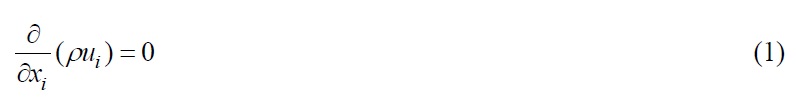
The present two-dimensional problem of wave-structure interaction is governed by the Navier-Stokes equations and continuity equation. Once the Reynolds averaging approach for turbulence modeling is applied, the Navier?Stokes equations can be written in Cartesian tensor form as
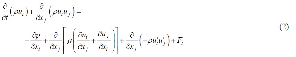
where
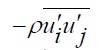
is the Reynolds stress term that was closed by using the standard
The equations of motion of a rectangular structure are expressed as follows,
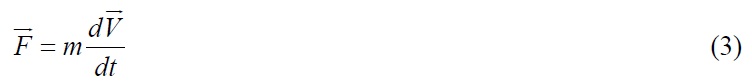

where
are the hydrodynamic force and the moment of the hydrodynamic force acting on the structure, respectively.
are the velocity and angular velocity of the floating structure, respectively. m is the mass of the structure,
In this study, the volume of fluid (VOF) method was employed to capture the free surface. The VOF method is popularly adopted to track and capture the free surface in two-phase problem. Also, most commercial computational fluid dynamics (CFD) codes use a variation of the VOF approach. In each cell, the volume fraction (
A cell with a
A single momentum equation is solved throughout the domain, and the resulting velocity field is shared among the phases (Hirt and Nichols, 1981). Convection and diffusion terms are discretized using the quadratic upstream interpolation for convective kinematics (QUICK) scheme and the second-order accurate central differencing scheme, respectively. For unsteady flow calculations, time derivative terms are discretized using the first-order accurate backward implicit scheme. The velocitypressure coupling and overall solution procedure are based on a pressure implicit with splitting of operators (PISO) algorithm adapted to the structured grid. The commercial CFD package, FLUENT (2010) was used for all numerical predictions in present study. Further details of the implementation can be found in the FLUENT (2010) manuals.
>
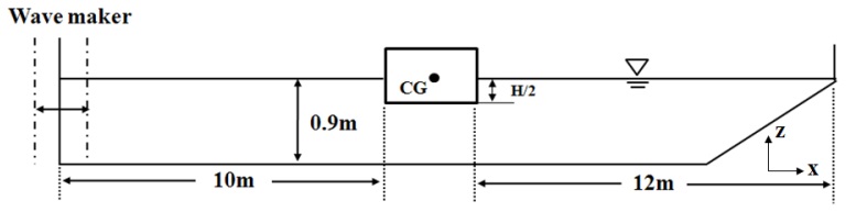
Computational domain and grid system
A rectangular structure 0.3
A piston-type wave generator was incorporated in the computational domain to generate the desired incident waves. The layering mesh technique, which is suitable for translation motion was used to move the piston. The piston motion was pure surge (translation in the x-direction only) and followed a the sinusoidal function given by

where
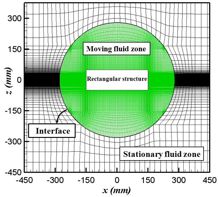
To simulate wave interaction with the structure, the sliding mesh technique was used to characterize the motion of the rectangular structure induced by fluid-structure interaction. Two independent grid systems were generated based on the structured grid as shown in Fig. 2. The moving fluid zone, including the rectangular structure, was allowed to rotate due to the moment caused by the hydrodynamic force acting on the structure. The stationary fluid zone was fixed. These two flow fields were interpolated each other through the interface by using a linear interpolation method. The grid was refined near the structure and the free surface to achieve better resolution of the flow field. Three different grid systems (coarse, medium and fine grids having 60,000, 100,000 and 150,000 grid cells, respectively) were considered to test the grid dependence of the solutions and to validate the present numerical methods. The dependence of the solutions on the grid systems considered in this study were not strong. Consequently, the medium grid system was selected for all cases.
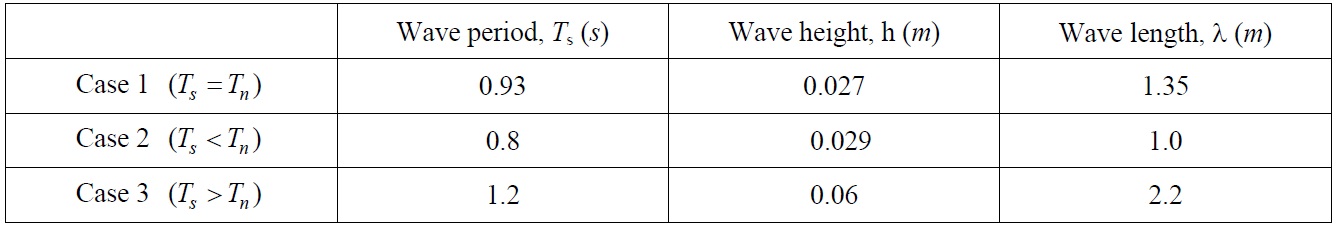
The present study considered three different wave periods that were shorter, equal to and longer than the roll natural period of the rectangular structure in order to observe the dependence of the flow structures around the rectangular floating structure and its roll motion on the wave period. The roll natural period of the structure was obtained by conducting a roll free decay test. Table 1 shows that the wave conditions used in present computation are the same as those used by Jung (2004b).

Wave conditions.
>
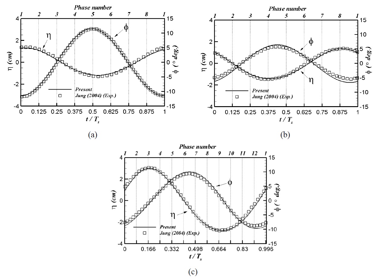
Wave and roll motion profiles
Fig. 3 shows a comparison of the profiles of wave elevation (
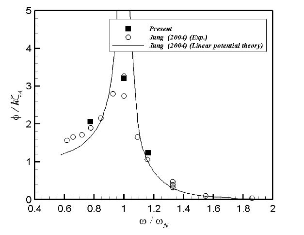
In the design of ship and other floating structures, a response amplitude operator (RAO) is an engineering statistic, or a set of such statistics, used to determine the likely behavior of a ship when operating at sea. RAOs are usually obtained using models of proposed ship designs tested in a model basin, or by running CFD programs, or from linear potential theory.
Fig. 4 shows a comparison of present RAOs with the experimental results and linear potential theory results by Jung (2004b) as a function of
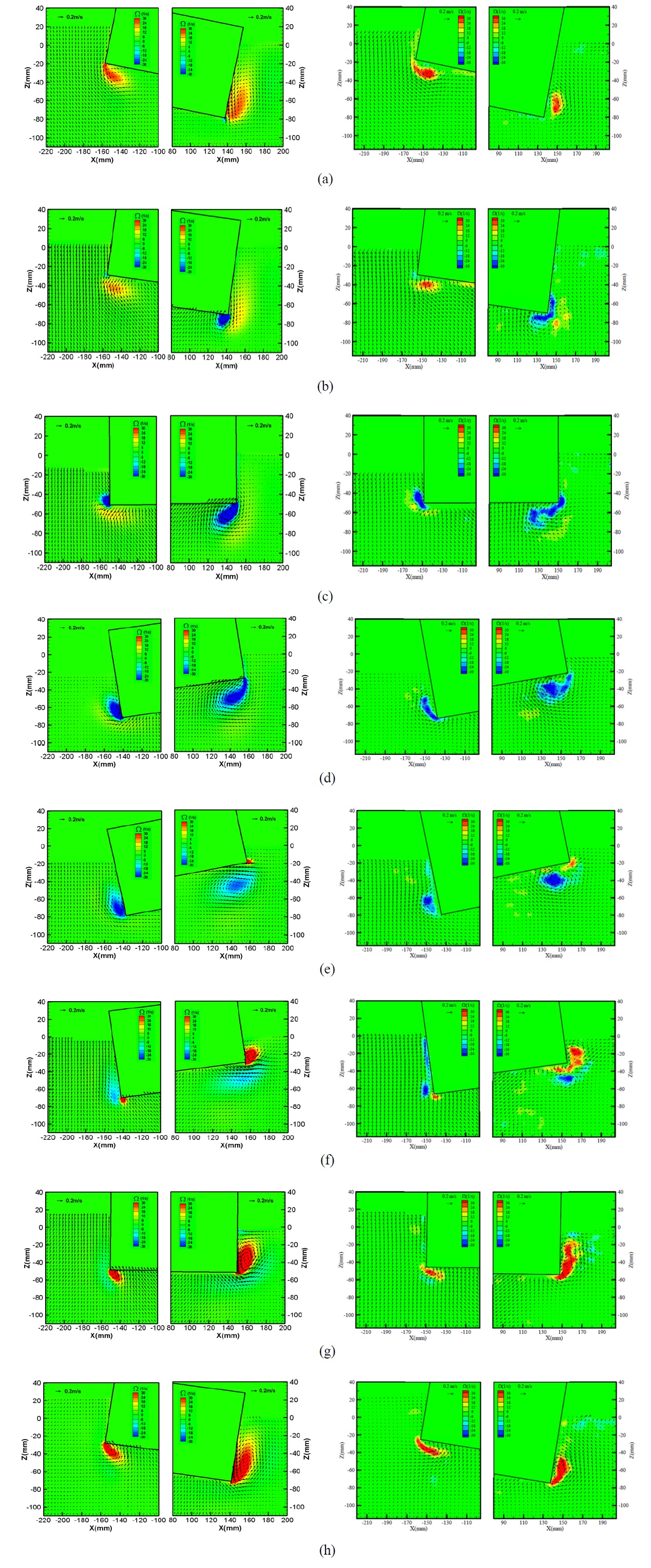
Fig. 5 shows the velocity vectors and vorticity contours of present numerical results and experimental results of Jung (2004b) according to phase, as shown in Fig. 3(a), for
In phase 2, the structure started to rotate counterclockwise. The magnitude of the rotational angle decreased with the negative value of
In phase 3, the structure is continuously rotating in the counterclockwise direction and is placed almost horizontally with a rotational angle of about 0° , as shown in Fig. 3(a). The clockwise rotating vortex appeared near the left side wall at the seaward bottom corner. On the leeward side, the clockwise rotating vortex that originated early in phase 2 increased in size and strength, as shown in Fig. 5(c). In phase 4, these clockwise rotating vortices on both sides kept augmenting with an increasing counterclockwise roll of the structure, Figs. 5(c) and (d). In phase 4, the positive vorticities near both sides also dissipated.
In phase 5, since the structure reached the extreme positive rotational angle as shown in Fig. 3(a), the clockwise rotating vortex near the right bottom corner on the leeward side of the structure moved further away from the structure. Subsequently, the negative vorticity became weak and separated from the left bottom corner, as shown in Fig. 5(e). This can be verified by comparing phase 4 in Fig. 5(d) and phase 5 in Fig. 5(e). Simultaneously, in the vicinity of the right corner on the leeward side, a tiny positive vorticity started to appear. On the seaward side, the negative vorticity accompanied by the clockwise rotating vortex near the left side corner also became weak in comparison to phase 4. In contrast to behavior on the leeward side, the positive vorticity did not exit at this phase on the seaward side.
The structure kept rotating clockwise, corresponding to phases 6, 7 and 8 shown in Figs. 5(f), (g) and (h), respectively. The positive vortex increased with increasing magnitude of the positive vorticity in the corner of the leeward side. The negative vorticity decreased and eventually disappeared near the bottom corner of the leeward side in phase 7, as shown in Fig. 5(g). A small positive vortex started to generate in the corner of the seaward side, starting its clockwise roll motion in phase 6 as shown in Fig. 5(f). Then, the positive vortex came into the larger vortex shape on the seaward side until the start of phase 8, as shown in Fig. 5(h).
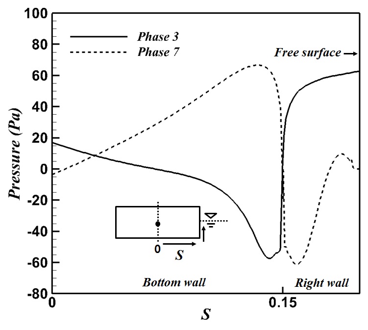
This entire process, described above, of the vortex generation and evolution was made by roll motion ahead of the fluid near the structure. Therefore, it caused the viscous damping effect, which reduces the roll motion with the roll natural period wave. This viscous damping effect related to the corner vortices is associated with the pressure force on the body and eventually the roll motion of the body. Thus, the pressure distribution on the body surface is plotted to identify the viscous damping effect on the force in Fig. 6 where considers representatively phase 3 and phase 7 corresponding to Figs. 5(c) and (g), respectively. In addition, the hydrostatic pressure is ignored to observe the net effect of the vortices and the right half of the body is only considered because of the almost symmetric relation between the left and right half.
In phase 3, the negative peak of the pressure near the right bottom corner distinctly appears as shown in Fig. 6, which is derived by the strong clockwise rotating vortex at this corner as observed in Fig. 5(c). In this phase, this negative pressure plays a role in damping the counterclockwise roll motion of the body.
In phase 7 in Fig. 6, the negative peak of the pressure occurs at the position near the right corner on the right side wall, which is associated with the strong counterclockwise rotating vortex at this region as shown in Fig. 5(g). This suction effect interrupts the clockwise roll motion of the body.
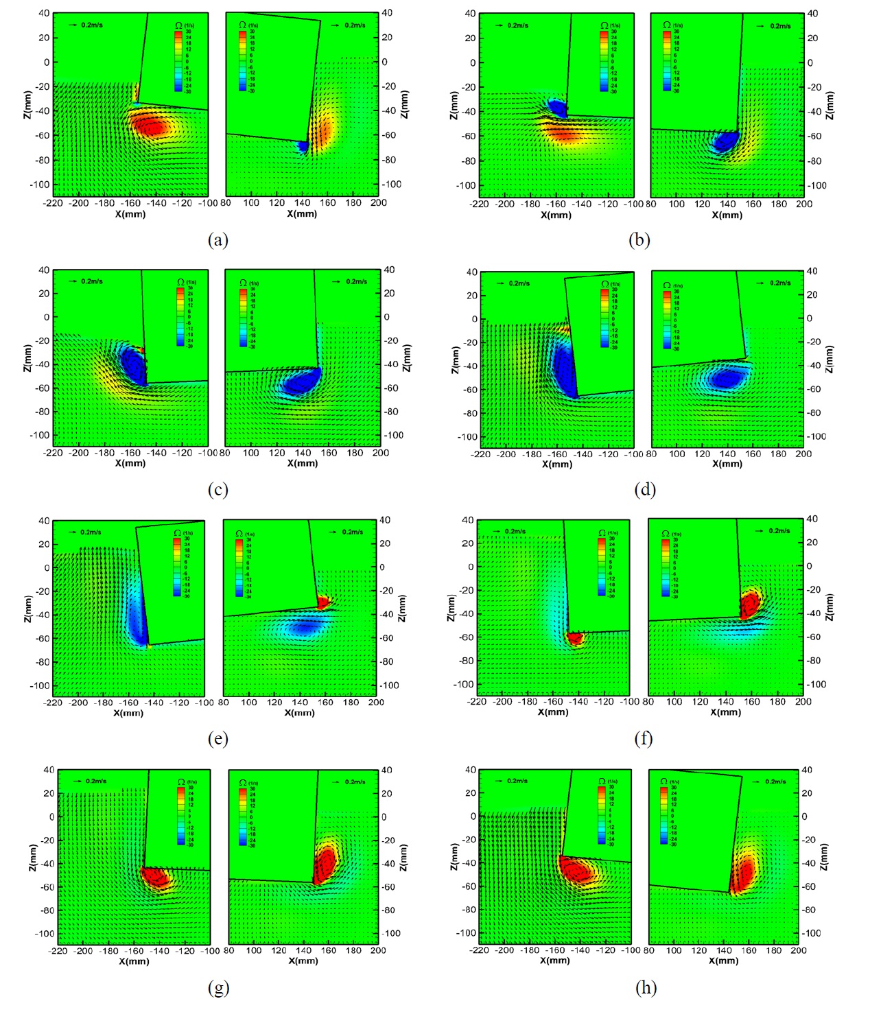
Fig. 7 shows the velocity vectors and vorticity contours at different phases for a wave period of
When the structure started to incline in the counterclockwise direction in phase 1 (Fig. 3(b)), a counterclockwise vortex with positive vorticity appeared to be most developed under the bottom of structure on the seaward side, as shown in Fig. 7(a). While
negative vorticity developed in a circular shape at the trough of a wave on the seaward side in phase 2, the negative vortex began to be separated by counterclockwise roll motion on the leeward side, as depicted in Fig. 7(b).
As the roll motion increased in the counterclockwise direction, the negative vortex with negative vorticity increased in size and strength on the seaward side. Also, the negative vortex near the right side bottom on the leeward side developed in phase 3 and phase 4, as shown in Figs. 7(c) and (d), respectively.
After passing the extreme positive rotational angle, the clockwise rotating vortex near the right bottom corner on the leeward side of the structure moved away from the structure with decreasing size and strength in phase 5, as shown in Fig. 7(e). However, a tiny positive vorticity appeared in the right corner on the leeward side. The clockwise rotating vortex on the seaward side decayed in this phase due to the clockwise roll motion.
Beyond phase 6, the clockwise roll motion accompanying the descending free surface contributed to the generation of a positive vortex on the seaward side as shown in Fig. 7(f). Also, the positive vortex was evolved by the roll motion as clarified in phases 7 and 8 in Figs. 7(g) and (h), respectively. On the leeward side, the positive vortex increased with increased magnitude of the positive vorticity in the corner with increased the roll motion in the clockwise direction, corresponding to phases 6, 7 and 8 in Figs. 7(f), (g) and (h), respectively.
At this wave period of
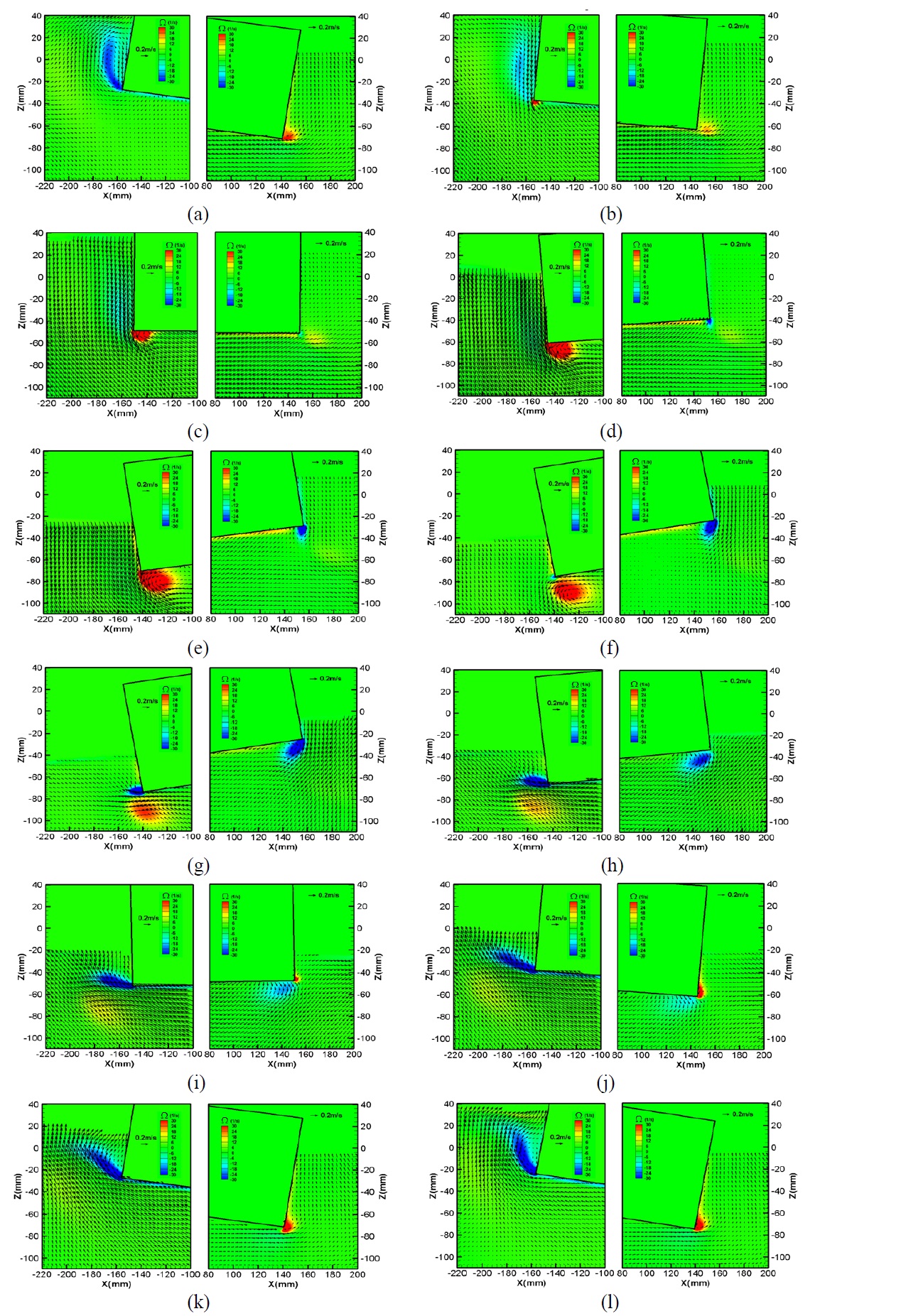
Fig. 8 shows the velocity vectors and the vorticity contours at different phases for a wave period of
However, with a longer wave of
When the structure rotated in the counterclockwise direction, corresponding to phases (1-6) as shown in Figs. 8(a)-(f), respectively, the free surface on the seaward side had the highest level in phase 2 and the incident wave was the crest in phase 3, which is shown on Fig. 3(c). On the seaward side the free surface descending to the minimum water level was faster than the rotation of the structure corner in the counterclockwise direction. Then, the positive vortex most developed with decaying the negative vortex under the structure on the seaward side with descending the water level. This vortex pattern is the opposite of those of the shorter wave periods of
At the corner of the leeward side, with the structure rotating in the counterclockwise direction, the remnant positive vortex decayed in phases (1-3) as shown in Figs. 8(a)-(c), respectively. However the negative vortex initiated in phase 4 (Fig. 8(d)) and increased in the phases (5-6) in Figs. 8(e)-(f), respectively. Thus, this comes to conclusion that the roll motion was predominant to the vortex evolution in the corner of the leeward side for the longer wave
When the structure rotated in the clockwise direction with the free surface ascending in phases (7-12) in Figs. 8(g)-(l), respectively, the negative vortex developed while the positive vortex dissipated away from the bottom corner on the seaward side. In contrast to the seaward side, the positive vortex developed while the negative vortex dissipated near the left bottom corner on the leeward side.
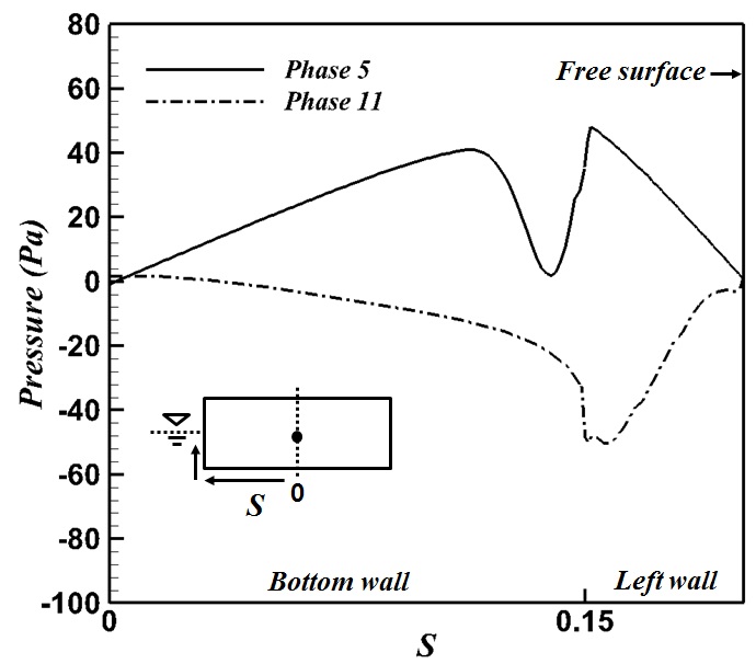
Fig. 9 shows the pressure distribution on the body surface in representatively phases 5 and 11 where the corresponding velocity field are in Figs. 8(e) and (k), respectively. Like Fig. 6, the hydrostatic pressure is ignored to observe the net effect of the vortices and the left half of the body is only considered. In phases 5 and 11, the low pressures appear near the left bottom corner and the position near the left corner on the left side wall, respectively, which are associated with the strong counterclockwise and clockwise rotating vortices at these regions as shown in Figs. Figs. 8(e) and (k). In these phases, these low pressures play a role in boosting the counterclockwise and clockwise roll motion of the body. This contribution of the corner vortices on the roll motion of the body at this
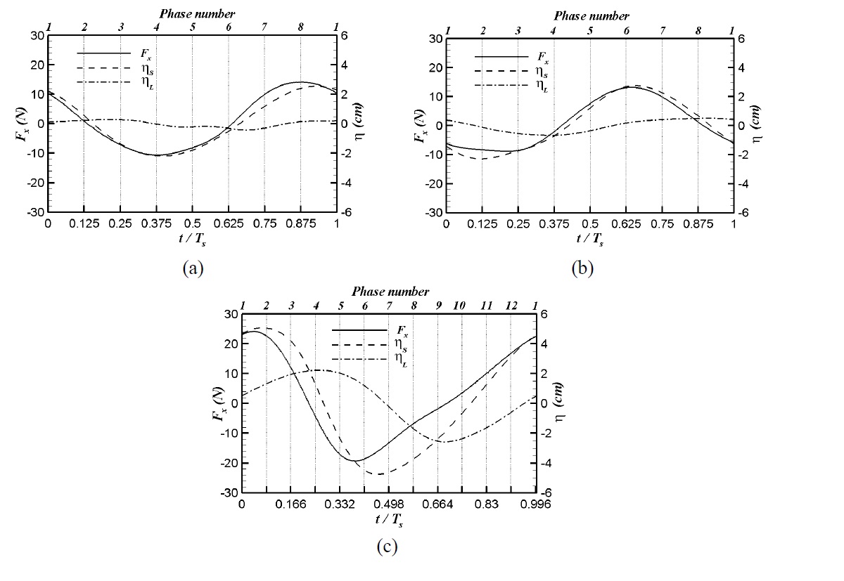
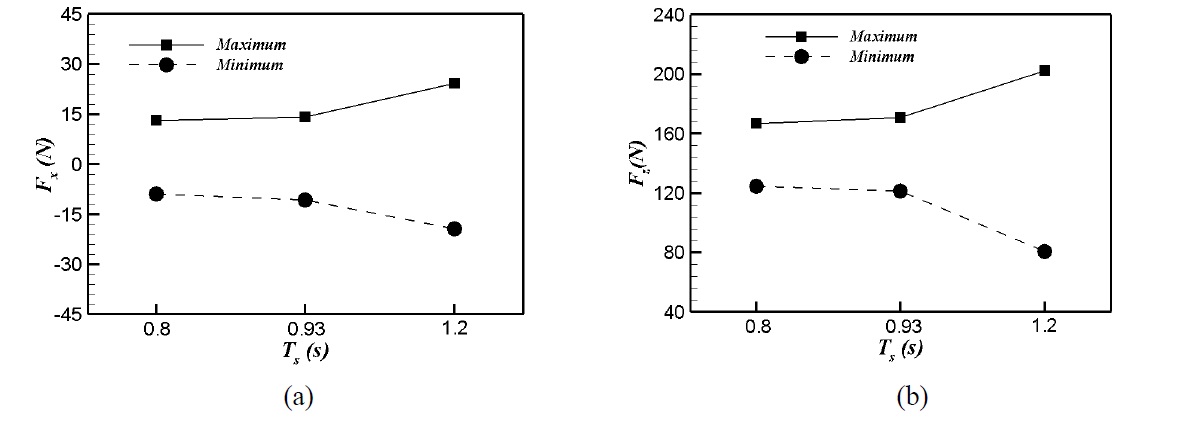
Fig. 10 shows the x-directional forces (
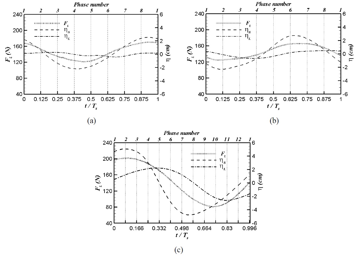
Fig. 11 shows the z-directional forces (
The maximum and minimum values of
This study numerically investigated the interaction of a regular wave and the roll motion of a rectangular floating structure. In order to simulate the two-dimensional (2D) incompressible viscous two-phase flow in a numerical wave tank with the rectangular floating structure, the present study used the volume of fluid (VOF) method based on the finite volume method. The sliding mesh technique was adopted to characterize the motion of the rectangular floating structure induced by fluid-structure interaction. The effects of the wave period on the flow, roll motion and forces acting on the structure were examined by considering three different wave periods that were shorter, equal to, and longer than roll natural period of the rectangular structure.
The time variations of the wave height and the roll motion of the rectangular structure are in good agreement with those of Jung’s experimental results (2004b) for all wave periods. The present RAOs compare well with the experimental results. Also, the present RAOs compare well with linear potential theory except at the natural frequency where the RAO based on theory is significantly magnified.
The present numerical results represented well the entire process of vortex generation and evolution presented by Jung (2004b). The shorter and natural wave periods revealed that the viscous damping effect reduced the roll motion. At a longer wave period, development of the vortex depended on the wave level instead of the roll motion shown in the shorter wave periods.
The x-directional forces were mainly governed by the difference in wave heights on the seaward and leeward sides. The time behavior of the z-directional forces was determined by the descent and the ascent of the wave. As the wave period increased beyond the natural wave period, the maximum and the minimum values of both forces rapidly increased.